Welcome to the nshap Package!

This is a python package to compute interaction indices that extend the Shapley Value. It accompanies the AISTATS'23 paper From Shapley Values to Generalized Additive Models and back by Sebastian Bordt and Ulrike von Luxburg.

This package supports, among others,

n-Shapley Values, introduced in our paper
SHAP Interaction Values, a popular interaction index that can also be computed with the shap package
the Shapley Taylor interaction index
the Faith-Shap interaction index
the Faith-Banzhaf interaction index.

The package works with arbitrary user-defined value functions. It also provides a model-agnostic implementation of the interventional SHAP value function.

Note that the computed interaction indices are an estimate that can be inaccurate, especially if the order of the interaction is large.

Documentation is available at https://tml-tuebingen.github.io/nshap.

⚠️ Disclaimer

This package does not provide an efficient way to compute Shapley Values. For this you should refer to the shap package or approaches like FastSHAP. In practice, the current implementation works for arbitrary functions of up to ~10 variables.

Setup

To install the package run

pip install nshap

Computing Interaction Indices

Let's assume that we have trained a Gradient Boosted Tree on the Folktables Income data set.

gbtree = xgboost.XGBClassifier()
gbtree.fit(X_train, Y_train)
print(f'Accuracy: {accuracy_score(Y_test, gbtree.predict(X_test)):0.3f}')

Accuracy: 0.830

Now we want to compute an interaction index. This package supports interaction indices that extend the Shapley Value. This means that the interaction index is based on a value function, just as the Shapley Value. So we need to define a value function. We can use the function nshap.vfunc.interventional_shap, which approximates the interventional SHAP value function.

import nshap

vfunc = nshap.vfunc.interventional_shap(gbtree.predict_proba, X_train, target=0, num_samples=1000)

The function takes 4 arguments

The function that we want to explain
The training data or another sample from the data distribution
The target class (required here since 'predict_proba' has 2 outputs).
The number of samples that should be used to estimate the expectation (Default: 1000)

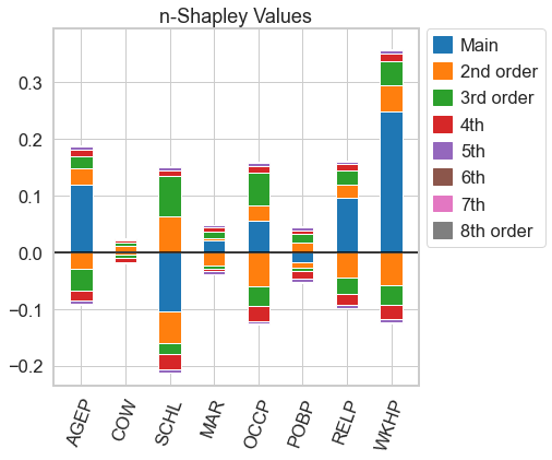
Equipped with a value function, we can compute different kinds of interaction indices. We can compute n-Shapley Values

n_shapley_values = nshap.n_shapley_values(X_test[0, :], vfunc, n=8)

the Shapley-Taylor interaction index

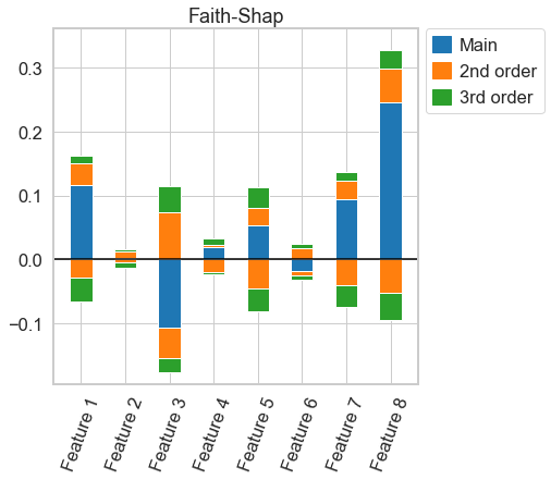
shapley_taylor = nshap.shapley_taylor(X_test[0, :], vfunc, n=8)

or the Faith-Shap interaction index of order 3

faith_shap = nshap.faith_shap(X_test[0, :], vfunc, n=3)

The functions that compute interaction indices have a common interface. They take 3 arguments

x: The data point for which to compute the explanation (numpy.ndarray)
v_func: The value function.
n: The order of the interaction index. Defaults to the number of features.

All functions return an object of type InteractionIndex. To get the interaction between features 2 and 3, simply call

n_shapley_values[(2,3)]

-0.0054

To visualize an interaction index, call

n_shapley_values.plot(feature_names = feature_names)

This works for all interaction indices

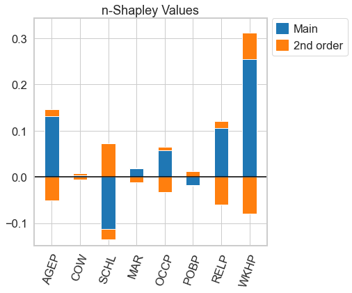
faith_shap.plot(feature_names = feature_names)

For n-Shapley Values, we can compute interaction indices of lower order from those of higher order

n_shapley_values.k_shapley_values(2).plot(feature_names = feature_names)

We can also obtain the original Shapley Values and plot them with the plotting functions from the shap package.

import shap

shap.force_plot(vfunc(X_test[0,:], []), n_shapley_values.shapley_values())

Let us compare our result to the Shapley Values obtained from the KernelSHAP Algorithm.

explainer = shap.KernelExplainer(gbtree.predict_proba, shap.kmeans(X_train, 25))
shap.force_plot(explainer.expected_value[0], shap_values[0])

The `InteractionIndex` class

The InteractionIndex class is a python dict with some added functionallity. It supports the following operations.

The individual attributions can be indexed with tuples of integers. For example, indexing with (0,) returns the main effect of the first feature. Indexing with (0,1,2) returns the interaction effect between features 0, 1 and 2.
plot() generates the plots described in the paper.
sum() sums the individual attributions (this does usually sum to the function value minus the value of the empty coalition)
save(fname) serializes the object to json. Can be loaded from there with nshap.load(fname). This can be useful since computing interaction indices takes time, so you might want to compute them in parallel, then aggregate the results for analysis.

Some function can only be called certain interaction indices:

k_shapley_values(k) computes the $k$-Shapley Values using the recursive relationship among $n$-Shapley Values of different order (requires $k\leq n$). Can only be called for $n$-Shapley Values.
shapley_values() returns the associated original Shapley Values as a list. Useful for compatiblity with the shap package.

Definig Value Functions

A value function has to follow the interface v_func(x, S) where x is a single data point (a numpy.ndarray) and S is a python list with the indices the the coordinates that belong to the coaltion.

In the introductory example with the Gradient Boosted Tree,

vfunc(x, [])

returns the expected predicted probability that an observation belongs to class 0, and

vfunc(x, [0,1,2,3,4,5,6,7])

returns the predicted probability that the observation x belongs to class 0 (note that the problem is 8-dimensional).

Implementation Details

At the moment all functions computes interaction indices simply via their definition. Independent of the order n of the $n$-Shapley Values, this requires to call the value function v_func once for all $2^d$ subsets of coordinates. Thus, the current implementation provides no essential speedup for the computation of $n$-Shapley Values of lower order.

The function nshap.vfunc.interventional_shap approximates the interventional SHAP value function by intervening on the coordinates of randomly sampled points from the data distributions.

Accuray of the computed interaction indices

The computed interaction indices are an estimate which can be inaccurate.

The estimation error depends on the precision of the value function. With the provided implementation of the interventional SHAP value function, the precision depends on the number of samples used to estimate the expectation.

A simple way to test whether your result is precisely estimated to increase the number of samples (the num_samples parameter of nshap.vfunc.interventional_shap) and see if the result changes.

For more details, check out the discussion in Section 8 of our paper.

Replicating the Results in our Paper

The folder notebooks\replicate-paper contains Jupyter Notebooks that allow to replicated the results in our paper.

The notebooks figures.ipynb and checkerboard-figures.ipynb generate all the figures in the paper.
The notebook estimation.ipynb provides the estimation example with the kNN classifier on the Folktables Travel data set that we discuss in Appendix Section B.
The notebook hyperparameters.ipynb cross-validates the parameter $k$ of the kNN classifier.
The notebooks compute.ipynb, compute-vfunc.ipynb, checkerboard-compute.ipynb and checkerboard-compute-million.ipynb compute the different $n$-Shapley Values. You do not have to run these notebooks, the pre-computed results can be downloaded here.

⚠️ Important

You have use version 0.1.0 of this package in order to run the notebooks that replicate the results in the paper.

pip install nshap=0.1.0

Citing nshap

If you use this software in your research, we encourage you to cite our paper.

@inproceedings{bordtlux2023,
  author    = {Bordt, Sebastian and von Luxburg, Ulrike},
  title     = {From Shapley Values to Generalized Additive Models and back},
  booktitle = {AISTATS},
  year      = {2023}
 }

If you use interaction indices that were introduced in other works, such as Shapley Taylor or Faith-Shap, you should also consider to cite the respective papers.

tml-tuebingen/nshap