P(i/y)thon h(i/y)stograms. Inspired (and based on) numpy.histogram, but designed for humans(TM) on steroids(TM).
The goal is to unify different concepts of histograms as occurring in numpy, pandas, matplotlib, ROOT, etc. and to create one representation that is easily manipulated with from the data point of view and at the same time provides nice integration into IPython notebook and various plotting options. In short, whatever you want to do with histograms, physt aims to be on your side.
Note: bokeh plotting backend has been discontinued (due to external library being redesigned.)
- Versions 0.3.x support Python 2.7 (no new releases in 2019)
- Versions 0.4.x support only Python 3.5+ while continuing the 0.3 API
- Versions 0.5.x will contain reworked API and will require Python 3.6
from physt import h1

# Create the sample
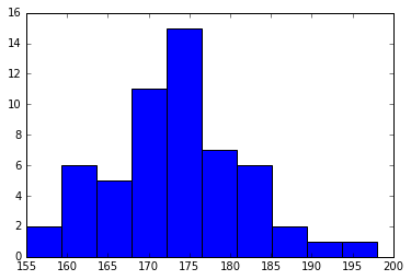
heights = [160, 155, 156, 198, 177, 168, 191, 183, 184, 179, 178, 172, 173, 175,
           172, 177, 176, 175, 174, 173, 174, 175, 177, 169, 168, 164, 175, 188,
           178, 174, 173, 181, 185, 166, 162, 163, 171, 165, 180, 189, 166, 163,
           172, 173, 174, 183, 184, 161, 162, 168, 169, 174, 176, 170, 169, 165]

hist = h1(heights, 10)           # <--- get the histogram data
hist << 190                      # <--- add a forgotten value
hist.plot() # <--- and plot itfrom physt import h2
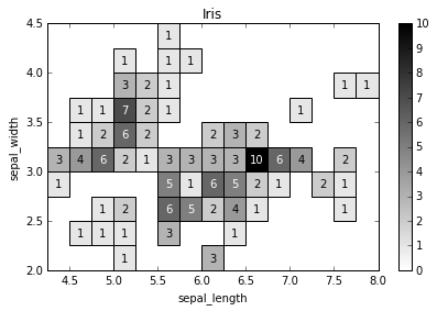
import seaborn as sns
iris = sns.load_dataset('iris')
iris_hist = h2(iris["sepal_length"], iris["sepal_width"], "human", (12, 7), name="Iris")
iris_hist.plot(show_zero=False, cmap="gray_r", show_values=True);import numpy as np
from physt import special
# Generate some sample data
data = np.empty((1000, 3))
data[:,0] = np.random.normal(0, 1, 1000)
data[:,1] = np.random.normal(0, 1.3, 1000)
data[:,2] = np.random.normal(1, .6, 1000)
# Get histogram data (in spherical coordinates)
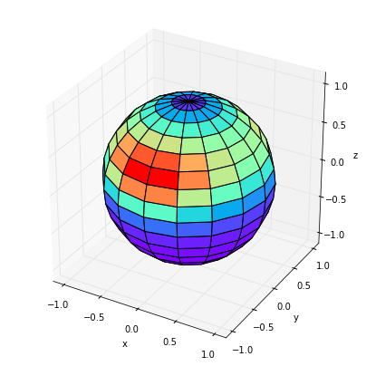
h = special.spherical_histogram(data)
# And plot its projection on a globe
h.projection("theta", "phi").plot.globe_map(density=True, figsize=(7, 7), cmap="rainbow") See more in docstring's and notebooks:
- Basic tutorial: http://nbviewer.jupyter.org/github/janpipek/physt/blob/master/doc/tutorial.ipynb
- Binning: http://nbviewer.jupyter.org/github/janpipek/physt/blob/master/doc/binning.ipynb
- 2D histograms: http://nbviewer.jupyter.org/github/janpipek/physt/blob/master/doc/2d_histograms.ipynb
- Special histograms (polar, spherical, cylindrical - beta): http://nbviewer.jupyter.org/github/janpipek/physt/blob/master/doc/special_histograms.ipynb
- Adaptive histograms: http://nbviewer.jupyter.org/github/janpipek/physt/blob/master/doc/adaptive_histogram.ipynb
- Use dask for large (not "big") data - alpha: http://nbviewer.jupyter.org/github/janpipek/physt/blob/master/doc/dask.ipynb
- Geographical bins . alpha: http://nbviewer.jupyter.org/github/janpipek/physt/blob/master/doc/geospatial.ipynb
- Plotting with vega backend: http://nbviewer.jupyter.org/github/janpipek/physt/blob/master/doc/vega-examples.ipynb
Using pip:
pip install physt
- 1D histograms
- 2D histograms
- ND histograms
- Some special histograms
- 2D polar coordinates (with plotting)
- 3D spherical / cylindrical coordinates (beta)
- Adaptive rebinning for on-line filling of unknown data (beta)
- Non-consecutive bins
- Memory-effective histogramming of dask arrays (beta)
- Understands any numpy-array-like object
- Keep underflow / overflow / missed bins
- Basic numeric operations (* / + -)
- Items / slice selection (including mask arrays)
- Add new values (fill, fill_n)
- Cumulative values, densities
- Simple statistics for original data (mean, std, sem)
- Plotting with several backends
- matplotlib (static plots with many options)
- vega (interactive plots, beta, help wanted!)
- folium (experimental for geo-data)
- plotly (very basic, help wanted!)
- ascii (experimental)
- Algorithms for optimized binning
- human-friendly
- mathematical
- IO, conversions
- I/O JSON
- I/O xarray.DataSet (experimental)
- I/O protobuf (experimental)
- O ROOT file (experimental)
- O pandas.DataFrame (basic)
- Rebinning
- using reference to original data?
- merging bins
- Statistics (based on original data)?
- Stacked histograms (with names)
- Potentially holoviews plotting backend (instead of the discontinued bokeh one)
- Kernel density estimates - use your favourite statistics package (like
seaborn) - Rebinning using interpolation - it should be trivial to use
rebin(https://github.com/jhykes/rebin) with physt
Rationale (for both): physt is dumb, but precise.
- Python 3.5+
- numpy
- (optional) matplotlib - simple output
- (optional) xarray - I/O
- (optional) protobuf - I/O
- (optional) uproot - I/O
- (optional) astropy - additional binning algorithms
- (optional) folium - map plotting
- (optional) vega3 - for vega in-line in IPython notebook (note that to generate vega JSON, this is not necessary)
- (optional) asciiplotlib - for ASCII bar plots
- (optional) xtermcolot - for ASCII color maps
- (testing) py.test, pandas
- (docs) sphinx, sphinx_rtd_theme, ipython
Talk at PyData Berlin 2018:
- https://janpipek.github.io/pydata2018-berlin/ - repository with slides and links
- https://www.youtube.com/watch?v=ZG-wH3-Up9Y - video of the talk
I am looking for anyone interested in using / developing physt. You can contribute by reporting errors, implementing missing features and suggest new one.
Thanks to:
- Ryan Mackenzie White - https://github.com/ryanmackenziewhite for the protobuf idea and first implementation
Patches:
- Matthieu Marinangeli - https://github.com/marinang


