This is a PROMISE Software Engineering Repository data set made publicly available in order to encourage repeatable, verifiable, refutable, and/or improvable predictive models of software engineering.
If you publish material based on PROMISE data sets then, please follow the acknowledgment guidelines posted on the PROMISE repository web page http://promise.site.uottawa.ca/SERepository .
Making decisions with a highly uncertain level is a critical problem in the area of software engineering. Predicting software quality requires high accurate tools and high-level experience. Otherwise, AI-based predictive models could be a useful tool with an accurate degree that helps on the prediction of software effort based on historical data from software development metrics. In this study, we built a software effort estimation model to predict this effort using a linear regression model. This statistical model was developed using a non-parametric linear regression algorithm based on the K-Nearest Neighbours (KNN). So, our results show the possibility of using AI methods to predict the software engineering effort prediction problem with an coefficient of determination of 76%
import math
from scipy.io import arff
from scipy.stats.stats import pearsonr
import pandas as pd
import numpy as np

from sklearn.linear_model import LinearRegression
from sklearn.neighbors import KNeighborsRegressor
from sklearn.model_selection import GridSearchCV
from sklearn.svm import SVR
from sklearn.model_selection import train_test_split

# Formatação mais bonita para os notebooks
import seaborn as sns
import matplotlib.pyplot as plt

%matplotlib inline
plt.style.use('fivethirtyeight')
plt.rcParams['figure.figsize'] = (15,5)
df_desharnais = pd.read_csv('../Datasets/02.desharnais.csv', header=0)
df_desharnais.head().dataframe tbody tr th {
vertical-align: top;
}
.dataframe thead th {
text-align: right;
}
| id | Project | TeamExp | ManagerExp | YearEnd | Length | Effort | Transactions | Entities | PointsNonAdjust | Adjustment | PointsAjust | Language | |
|---|---|---|---|---|---|---|---|---|---|---|---|---|---|
| 0 | 1 | 1 | 1 | 4 | 85 | 12 | 5152 | 253 | 52 | 305 | 34 | 302 | 1 |
| 1 | 2 | 2 | 0 | 0 | 86 | 4 | 5635 | 197 | 124 | 321 | 33 | 315 | 1 |
| 2 | 3 | 3 | 4 | 4 | 85 | 1 | 805 | 40 | 60 | 100 | 18 | 83 | 1 |
| 3 | 4 | 4 | 0 | 0 | 86 | 5 | 3829 | 200 | 119 | 319 | 30 | 303 | 1 |
| 4 | 5 | 5 | 0 | 0 | 86 | 4 | 2149 | 140 | 94 | 234 | 24 | 208 | 1 |
df_desharnais.info()<class 'pandas.core.frame.DataFrame'>
RangeIndex: 81 entries, 0 to 80
Data columns (total 13 columns):
id 81 non-null int64
Project 81 non-null int64
TeamExp 81 non-null int64
ManagerExp 81 non-null int64
YearEnd 81 non-null int64
Length 81 non-null int64
Effort 81 non-null int64
Transactions 81 non-null int64
Entities 81 non-null int64
PointsNonAdjust 81 non-null int64
Adjustment 81 non-null int64
PointsAjust 81 non-null int64
Language 81 non-null int64
dtypes: int64(13)
memory usage: 8.3 KB
df_desharnais.describe().dataframe tbody tr th {
vertical-align: top;
}
.dataframe thead th {
text-align: right;
}
| id | Project | TeamExp | ManagerExp | YearEnd | Length | Effort | Transactions | Entities | PointsNonAdjust | Adjustment | PointsAjust | Language | |
|---|---|---|---|---|---|---|---|---|---|---|---|---|---|
| count | 81.000000 | 81.000000 | 81.000000 | 81.000000 | 81.000000 | 81.000000 | 81.000000 | 81.000000 | 81.000000 | 81.000000 | 81.000000 | 81.000000 | 81.000000 |
| mean | 41.000000 | 41.000000 | 2.185185 | 2.530864 | 85.740741 | 11.666667 | 5046.308642 | 182.123457 | 122.333333 | 304.456790 | 27.629630 | 289.234568 | 1.555556 |
| std | 23.526581 | 23.526581 | 1.415195 | 1.643825 | 1.222475 | 7.424621 | 4418.767228 | 144.035098 | 84.882124 | 180.210159 | 10.591795 | 185.761088 | 0.707107 |
| min | 1.000000 | 1.000000 | -1.000000 | -1.000000 | 82.000000 | 1.000000 | 546.000000 | 9.000000 | 7.000000 | 73.000000 | 5.000000 | 62.000000 | 1.000000 |
| 25% | 21.000000 | 21.000000 | 1.000000 | 1.000000 | 85.000000 | 6.000000 | 2352.000000 | 88.000000 | 57.000000 | 176.000000 | 20.000000 | 152.000000 | 1.000000 |
| 50% | 41.000000 | 41.000000 | 2.000000 | 3.000000 | 86.000000 | 10.000000 | 3647.000000 | 140.000000 | 99.000000 | 266.000000 | 28.000000 | 255.000000 | 1.000000 |
| 75% | 61.000000 | 61.000000 | 4.000000 | 4.000000 | 87.000000 | 14.000000 | 5922.000000 | 224.000000 | 169.000000 | 384.000000 | 35.000000 | 351.000000 | 2.000000 |
| max | 81.000000 | 81.000000 | 4.000000 | 7.000000 | 88.000000 | 39.000000 | 23940.000000 | 886.000000 | 387.000000 | 1127.000000 | 52.000000 | 1116.000000 | 3.000000 |
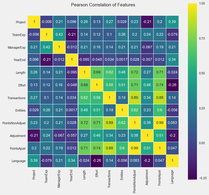
In this section, the correlations between attributes of Desharnais dataset and software effort are analyzed and applicability of the regression analysis is examined. The correlation between two variables is a measure of how well the variables are related. The most common measure of correlation in statistics is the Pearson Correlation (or the Pearson Product Moment Correlation - PPMC) which shows the linear relationship between two variables.
Pearson correlation coefficient analysis produces a result between -1 and 1. A result of -1 means that there is a perfect negative correlation between the two values at all, while a result of 1 means that there is a perfect positive correlation between the two variables.
Results between 0.5 and 1.0 indicate high correlation.Correlation coefficients are used in statistics to measure how strong a relationship is between two variables. There are several types of correlation coefficient. Pearson’s correlation (also called Pearson’s R) is a correlation coefficient commonly used in linear regression.
df_desharnais.corr().dataframe tbody tr th {
vertical-align: top;
}
.dataframe thead th {
text-align: right;
}
| id | Project | TeamExp | ManagerExp | YearEnd | Length | Effort | Transactions | Entities | PointsNonAdjust | Adjustment | PointsAjust | Language | |
|---|---|---|---|---|---|---|---|---|---|---|---|---|---|
| id | 1.000000 | 1.000000 | -0.006007 | 0.214294 | 0.096486 | 0.255187 | 0.126153 | 0.265891 | 0.028787 | 0.226076 | -0.207774 | 0.202608 | 0.391475 |
| Project | 1.000000 | 1.000000 | -0.006007 | 0.214294 | 0.096486 | 0.255187 | 0.126153 | 0.265891 | 0.028787 | 0.226076 | -0.207774 | 0.202608 | 0.391475 |
| TeamExp | -0.006007 | -0.006007 | 1.000000 | 0.424687 | -0.210335 | 0.143948 | 0.119529 | 0.103768 | 0.256608 | 0.203805 | 0.235629 | 0.222884 | -0.079112 |
| ManagerExp | 0.214294 | 0.214294 | 0.424687 | 1.000000 | -0.011519 | 0.211324 | 0.158303 | 0.138146 | 0.206644 | 0.207748 | -0.066821 | 0.187399 | 0.205521 |
| YearEnd | 0.096486 | 0.096486 | -0.210335 | -0.011519 | 1.000000 | -0.095027 | -0.048367 | 0.034331 | 0.001686 | 0.028234 | -0.056743 | 0.012106 | 0.342233 |
| Length | 0.255187 | 0.255187 | 0.143948 | 0.211324 | -0.095027 | 1.000000 | 0.693280 | 0.620711 | 0.483504 | 0.723849 | 0.266086 | 0.714092 | -0.023810 |
| Effort | 0.126153 | 0.126153 | 0.119529 | 0.158303 | -0.048367 | 0.693280 | 1.000000 | 0.581881 | 0.510328 | 0.705449 | 0.463865 | 0.738271 | -0.261942 |
| Transactions | 0.265891 | 0.265891 | 0.103768 | 0.138146 | 0.034331 | 0.620711 | 0.581881 | 1.000000 | 0.185041 | 0.886419 | 0.341906 | 0.880923 | 0.136778 |
| Entities | 0.028787 | 0.028787 | 0.256608 | 0.206644 | 0.001686 | 0.483504 | 0.510328 | 0.185041 | 1.000000 | 0.618913 | 0.234747 | 0.598401 | -0.056439 |
| PointsNonAdjust | 0.226076 | 0.226076 | 0.203805 | 0.207748 | 0.028234 | 0.723849 | 0.705449 | 0.886419 | 0.618913 | 1.000000 | 0.383842 | 0.985945 | 0.082737 |
| Adjustment | -0.207774 | -0.207774 | 0.235629 | -0.066821 | -0.056743 | 0.266086 | 0.463865 | 0.341906 | 0.234747 | 0.383842 | 1.000000 | 0.513197 | -0.199167 |
| PointsAjust | 0.202608 | 0.202608 | 0.222884 | 0.187399 | 0.012106 | 0.714092 | 0.738271 | 0.880923 | 0.598401 | 0.985945 | 0.513197 | 1.000000 | 0.046672 |
| Language | 0.391475 | 0.391475 | -0.079112 | 0.205521 | 0.342233 | -0.023810 | -0.261942 | 0.136778 | -0.056439 | 0.082737 | -0.199167 | 0.046672 | 1.000000 |
colormap = plt.cm.viridis
plt.figure(figsize=(10,10))
plt.title('Pearson Correlation of Features', y=1.05, size=15)
sns.set(font_scale=1.05)
sns.heatmap(df_desharnais.drop(['id'], axis=1).astype(float).corr(),linewidths=0.1,vmax=1.0, square=True,cmap=colormap, linecolor='white', annot=True)
<matplotlib.axes._subplots.AxesSubplot at 0x116178cc0>
features = [ 'TeamExp', 'ManagerExp', 'YearEnd', 'Length', 'Transactions', 'Entities',
        'PointsNonAdjust', 'Adjustment', 'PointsAjust']

max_corr_features = ['Length', 'Transactions', 'Entities','PointsNonAdjust','PointsAjust']

X = df_desharnais[max_corr_features]
y = df_desharnais['Effort']In this study the following algorithms were used: Linear Regression and K-Nearest Neighbors Regression. The training of the regressors models were performed on 67% of the instances
The K-Nearest Neighbor Regression is a simple algorithm that stores all available cases and predict the numerical target based on a similarity measure and it’s been used in a statistical estimation and pattern recognition as non-parametric technique classifying correctly unknown cases calculating euclidean distance between data points. In fact our choice by K-Nearest Neighbor Regression was motivated by the absence of a detailed explanation about how effort attribute value is calculated on Desharnais dataset. In the K-Nearest Neighbor Regression we choose to specify only 3 neighbors for k-neighbors queries and uniform weights, that means all points in each neighborhood are weighted equally.
X_train, X_test, y_train, y_test = train_test_split(X, y, test_size=0.33, random_state=30)

neigh = KNeighborsRegressor(n_neighbors=3, weights='uniform')
neigh.fit(X_train, y_train)
print(neigh.score(X_test, y_test))
0.7379861869550943
The regression analysis aims to verify the existence of a functional relationship between a variable with one or more variables, obtaining an equation that explains the variation of the dependent variable Y, by the variation of the levels of the independent variables. The training of the Linear Regression model consists of generating a regression for the target variable Y.
X_train, X_test, y_train, y_test = train_test_split(X, y, test_size=0.33, random_state=22)

model = LinearRegression()
model.fit(X_train, y_train)
print(model.score(X_test, y_test))
0.7680074954440712
X_train, X_test, y_train, y_test = train_test_split(X, y, test_size=0.33, random_state=22)

parameters = {'kernel':('linear', 'rbf'), 'C':[1,2,3,4,5,6,7,8,9,10]}

svr = SVR()
LinearSVC = GridSearchCV(svr, parameters)
LinearSVC.fit(X_train, y_train)
print("Best params hash: {}".format(LinearSVC.best_params_))
print(LinearSVC.score(X_test, y_test))
Best params hash: {'C': 1, 'kernel': 'linear'}
0.735919788126071
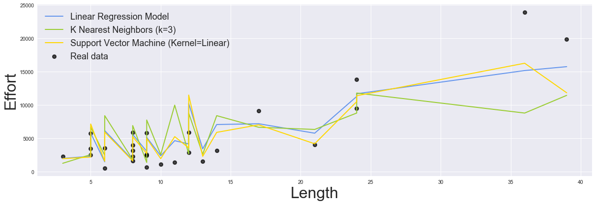
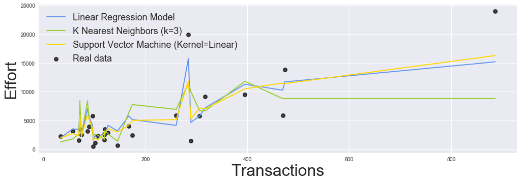
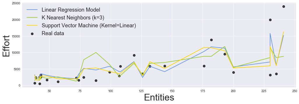
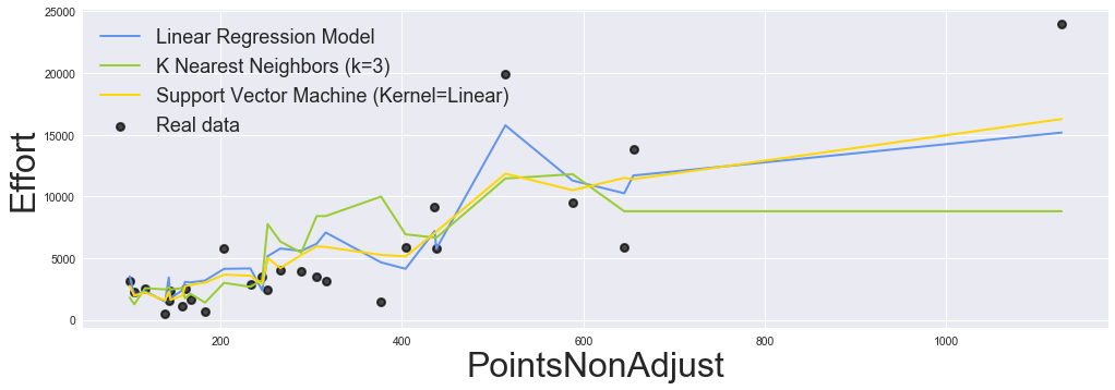
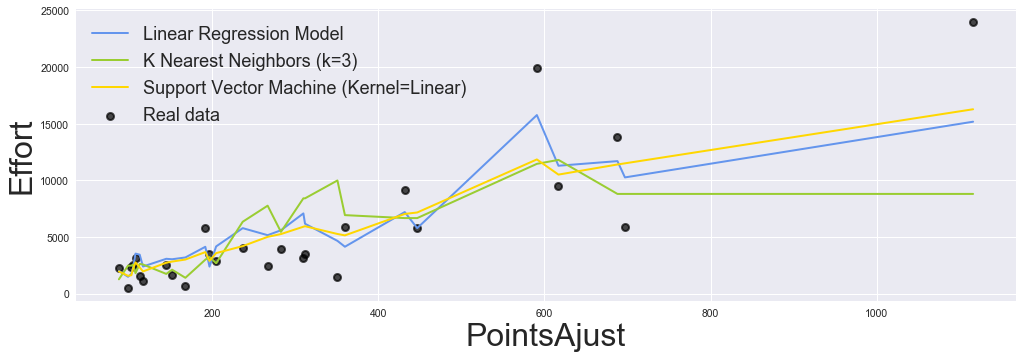
The figure shows the linear model (blue line) prediction is fairly close to Knn model effort prediction (red line), predicting the numerical target based on a similarity measure. According to the plot we observe that Linear Regression model (blue line) presents a better performance. Although Knn Regression model (red line) is fairly close to data points, the Linear Regression model shows a smaller mean squared error. It is possible to observe that the lines of both models present a slight tendency to rise, which justifies their correlation with the increase in effort. Some metrics are also highlighted by the presence of outliers.
plt.figure(figsize=(18,6))
plt.rcParams['legend.fontsize'] = 18
plt.rcParams['legend.loc']= 'upper left'
plt.rcParams['axes.labelsize']= 32

for i, feature in enumerate(max_corr_features):

    # Knn Regression Model
    xs, ys = zip(*sorted(zip(X_test[feature], neigh.fit(X_train, y_train).predict(X_test))))

    # Linear Regression Model
    model_xs, model_ys = zip(*sorted(zip(X_test[feature], model.fit(X_train, y_train).predict(X_test))))

    # Support Vector Machine
    svc_model_xs, svc_model_ys = zip(*sorted(zip(X_test[feature], LinearSVC.fit(X_train, y_train).predict(X_test))))

    plt.scatter(X_test[feature], y_test, label='Real data', lw=2,alpha= 0.7, c='k' )
    plt.plot(model_xs, model_ys , lw=2, label='Linear Regression Model', c='cornflowerblue')
    plt.plot(xs, ys , lw=2,label='K Nearest Neighbors (k=3)', c='yellowgreen')
    plt.plot(svc_model_xs, svc_model_ys , lw=2,label='Support Vector Machine (Kernel=Linear)', c='gold')

    plt.xlabel(feature)
    plt.ylabel('Effort')
    plt.legend()
    plt.show()