tonyduan/mixture-density-network

Mixture density network implemented in PyTorch.

Mixture Density Network

Last update: December 2022.

---

Lightweight implementation of a mixture density network [1] in PyTorch.

Setup

Suppose we want to regress response $\mathbf{y} \in \mathbb{R}^{d}$ using covariates $\mathbf{x} \in \mathbb{R}^n$.

We model the conditional distribution as a mixture of Gaussians

$$p_\theta(\mathbf{y}|\mathbf{x}) = \sum_{k=1}^K \pi_k N(\boldsymbol\mu^{(k)}, {\boldsymbol\Sigma}^{(k)}),$$

where the mixture distribution parameters are output by a neural network dependent on $\mathbf{x}$.

$$\begin{align*} ( \boldsymbol\pi & \in\Delta^{K-1} & \boldsymbol\mu^{(k)}&\in\mathbb{R}^{d} &\boldsymbol\Sigma^{(k)}&\in \mathrm{S}_+^d) = f_\theta(\mathbf{x}) \end{align*}$$

The training objective is to maximize log-likelihood. The objective is clearly non-convex.

$$\begin{align*} \log p_\theta(\mathbf{y}|\mathbf{x}) & \propto\log \sum_{k}\left(\pi_k\exp\left(-\frac{1}{2}\left(\mathbf{y}-\boldsymbol\mu^{(k)}\right)^\top {\boldsymbol\Sigma^{(k)}}^{-1}\left(\mathbf{y}-\boldsymbol\mu^{(k)}\right) -\frac{1}{2}\log\det \boldsymbol\Sigma^{(k)}\right)\right)\\\ & = \mathrm{logsumexp}_k\left(\log\pi_k - \frac{1}{2}\left(\mathbf{y}-\boldsymbol\mu^{(k)}\right)^\top {\boldsymbol\Sigma^{(k)}}^{-1}\left(\mathbf{y}-\boldsymbol\mu^{(k)}\right) -\frac{1}{2}\log\det \boldsymbol\Sigma^{(k)}\right)\\\ \end{align*}$$

Importantly, we need to use torch.log_softmax(...) to compute logits $\log \boldsymbol\pi$ for numerical stability.

Noise Model

There are several options we can make to constrain the noise model $\boldsymbol\Sigma^{(k)}$.

1. No assumptions, $\boldsymbol\Sigma^{(k)} \in \mathrm{S}_+^d$.
2. Fully factored, let $\boldsymbol\Sigma^{(k)} = \mathrm{diag}({\boldsymbol\sigma^{(k)}}^{2}), {\boldsymbol\sigma^{(k)}}^{2}\in\mathbb{R}_+^d$ where the noise level for each dimension is predicted separately.
3. Isotrotopic, let $\boldsymbol\Sigma^{(k)} = {\sigma^{(k)}}^{2}\mathbf{I}, {\sigma^{(k)}}^{2}\in\mathbb{R}_+$ which assumes the same noise level for each dimension over $d$.
4. Isotropic across clusters, let $\boldsymbol\Sigma^{(k)} = \sigma^2\mathbf{I}, \sigma^2\in\mathbb{R}_+$ which assumes the same noise level for each dimension over $d$ and cluster.
5. Fixed isotropic, same as above but do not learn $\sigma^2$.

Thse correspond to the following objectives.

$$\begin{align*} \log p_\theta(\mathbf{y}|\mathbf{x}) & = \mathrm{logsumexp}_k\left(\log\pi_k - \frac{1}{2}\left(\mathbf{y}-\boldsymbol\mu^{(k)}\right)^\top {\boldsymbol\Sigma^{(k)}}^{-1}\left(\mathbf{y}-\boldsymbol\mu^{(k)}\right) -\frac{1}{2}\log\det \boldsymbol\Sigma^{(k)}\right) \tag{1}\\\ & = \mathrm{logsumexp}_k \left(\log\pi_k - \frac{1}{2}\left\|\frac{\mathbf{y}-\boldsymbol\mu^{(k)}}{\boldsymbol\sigma^{(k)}}\right\|^2-\|\log\boldsymbol\sigma^{(k)}\|_1\right) \tag{2}\\\ & = \mathrm{logsumexp}_k \left(\log\pi_k - \frac{1}{2}\left\|\frac{\mathbf{y}-\boldsymbol\mu^{(k)}}{\sigma^{(k)}}\right\|^2-d\log(\sigma^{(k)})\right) \tag{3}\\\ & = \mathrm{logsumexp}_k \left(\log\pi_k - \frac{1}{2}\left\|\frac{\mathbf{y}-\boldsymbol\mu^{(k)}}{\sigma}\right\|^2-d\log(\sigma)\right) \tag{4}\\\ & = \mathrm{logsumexp}_k \left(\log\pi_k - \frac{1}{2}\left\|\frac{\mathbf{y}-\boldsymbol\mu^{(k)}}{\sigma}\right\|^2\right) \tag{5} \end{align*}$$

In this repository we implement options (2, 3, 4, 5).

Miscellaneous

Recall that the objective is clearly non-convex. For example, one local minimum is to ignore all modes except one and place a single diffuse Gaussian distribution on the marginal outcome (i.e. high ${\sigma}^{(k)}$).

For this reason it's often preferable to over-parameterize the model and specify n_components higher than the true hypothesized number of modes.

Usage

import torch
from src.blocks import MixtureDensityNetwork

x = torch.randn(5, 1)
y = torch.randn(5, 1)

# 1D input, 1D output, 3 mixture components
model = MixtureDensityNetwork(1, 1, n_components=3, hidden_dim=50)
pred_parameters = model(x)

# use this to backprop
loss = model.loss(x, y)

# use this to sample a trained model
samples = model.sample(x)

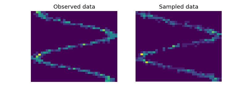
For further details see the examples/ folder. Below is a model fit with 3 components in ex_1d.py.

References

[1] Bishop, C. M. Mixture density networks. (1994).

[2] Ha, D. & Schmidhuber, J. Recurrent World Models Facilitate Policy Evolution. in Advances in Neural Information Processing Systems 31 (eds. Bengio, S. et al.) 2450–2462 (Curran Associates, Inc., 2018).

License

This code is available under the MIT License.