This repository contains the PyTorch implementation of our paper:
"SOLAR: Second-Order Loss and Attention for Image Retrieval"
Tony Ng, Vassileios Balntas, Yurun Tian, Krystian Mikolajczyk. ECCV 2020.
[arXiv] [short video] [long video] [ECCV Daily feature article] [OpenCV blog]
Before going further, please check out Filip Radenovic's great repository on image retrieval. Our solar-global module is heavily built upon it. If you use this code in your research, please also cite their work!
[link to license]
- Complete test scripts for large-scale image retrieval with
solar-global - Inference code for extracting local descriptors with
solar-local - Second-order attention map visualisation for large images
- Image matching visualisation
- Training code for image retrieval
- Python 3
- PyTorch tested on 1.3.0 - 1.5.1, torchvision 0.5+
- opencv-python (cv2) tested on 3.3.0.10
- TensorBoard tested on 2.0.0+
- numpy
- PIL
- tqdm
Begin with downloading our best models (both global and local) described in the paper, as well as the pre-computed descriptors of the 1M distractors set.
sh download.shThe global model is saved at data/networks/resnet101-solar-best.pth and the local model at solar_local/weights/local-solar-345-liberty.pth. The descriptors of the 1M distractors are saved in the main directory (the file is quite big ~8GB, so it might take a while to download).
Here you can try out our pretrained model resnet101-solar-best.pth on the Revisiting Oxford and Paris dataset
Testing on R-Oxford, R-Paris
Once you've successfully downloaded the global model weights, run
python3 -m solar_global.examples.test
This script automatically downloads roxford5k,rparis6k into data/test/ and evaluates SOLAR on them.
After a while, you should be able to get results as below
>> roxford5k: mAP E: 85.88, M: 69.9, H: 47.91
>> roxford5k: mP@k[1, 5, 10] E: [94.12 92.45 88.8 ], M: [94.29 90.86 86.71], H: [88.57 74.29 63.  ]

>> rparis6k: mAP E: 92.95, M: 81.57, H: 64.45
>> rparis6k: mP@k[1, 5, 10] E: [100.   96.57 95.43], M: [100.   98.   97.14], H: [97.14 94.57 93.  ]
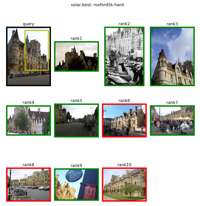
Retrieval rankings are visualised in specs/ using
tensorboard --logdir specs/ --samples_per_plugin images=1000You can view them on your browser at localhost:6006 in the IMAGES tab. Here's an example
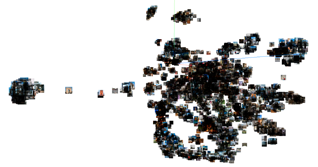
You can also switch to the PROJECTOR tab and play around with TensorBoard's embedding visualisation tool. Here's an example of the 6322 database images in R-Paris, visualised with t-SNE
Testing with the extra 1-million distractors
If you decide to extract the descriptors on your own, run
(Note: this step takes a lot of time and storage, and we only provide it for verification. You can skip to the next command if you've already downloded the pre-computed descriptors from the previous step!)
python3 -m solar_global.examples.extract_1m
This script would download and extract the 1M distractors set and save them into data/test/revisitop1m/. This dataset is quite large (400GB+), so depending on your network & GPU, the whole process of downloading + extracting descriptors can take from a couple of days to a week. In our setting (~100MBps, V100), the download + extraction takes ~10 hours and the descriptors ~30 hours to be computed.
Now, make sure that resnet101-solar-best.pth_vecs_revisitop1m.pt is in the main directory, whether from the extraction step above or from the download ealier. Then you can run
python3 -m solar_global.examples.test_1m
and get results as below
>> roxford5k: mAP E: 72.04, M: 53.49, H: 29.89
>> roxford5k: mP@k[1, 5, 10] E: [88.24 81.99 76.96], M: [88.57 82.29 76.71], H: [74.29 58.29 48.86]

>> rparis6k: mAP E: 83.35, M: 59.19, H: 33.41
>> rparis6k: mP@k[1, 5, 10] E: [98.57 95.14 93.57], M: [98.57 96.29 94.86], H: [92.86 89.14 81.57]
Using our interactive visualisation tool
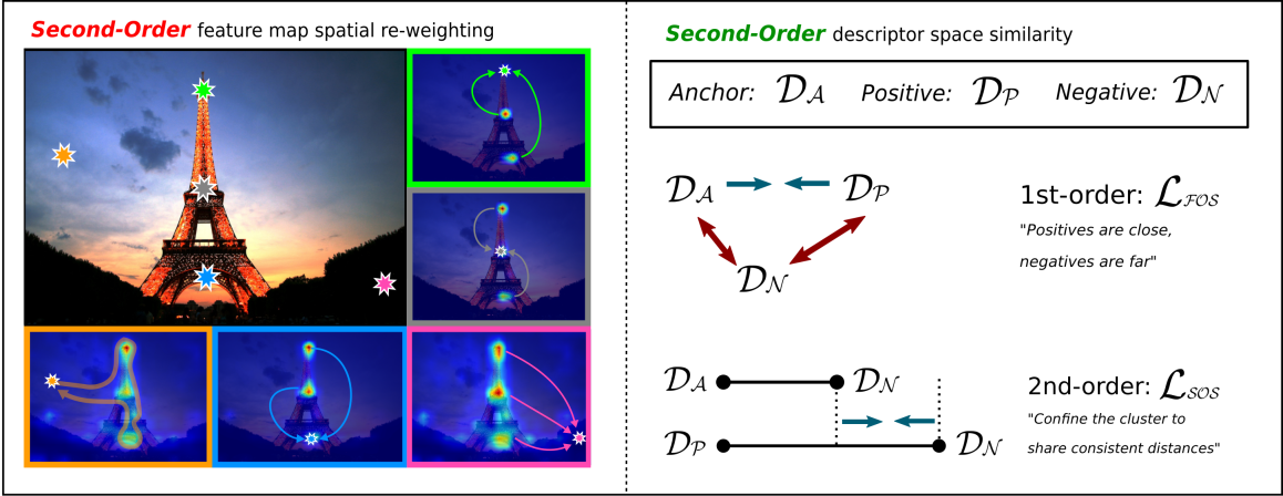
We provide a small demo for you to click around an image and interactively visualise the second-order attention (SOA) maps at different locations you select. (c.f. Section 4.3 in the paper for an in-depth analysis)
First, run
python3 -m demo.interactive_soa
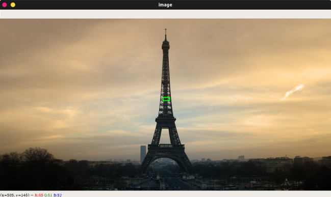
This gorgeous image of the Eiffel Tower should pop up in a new window
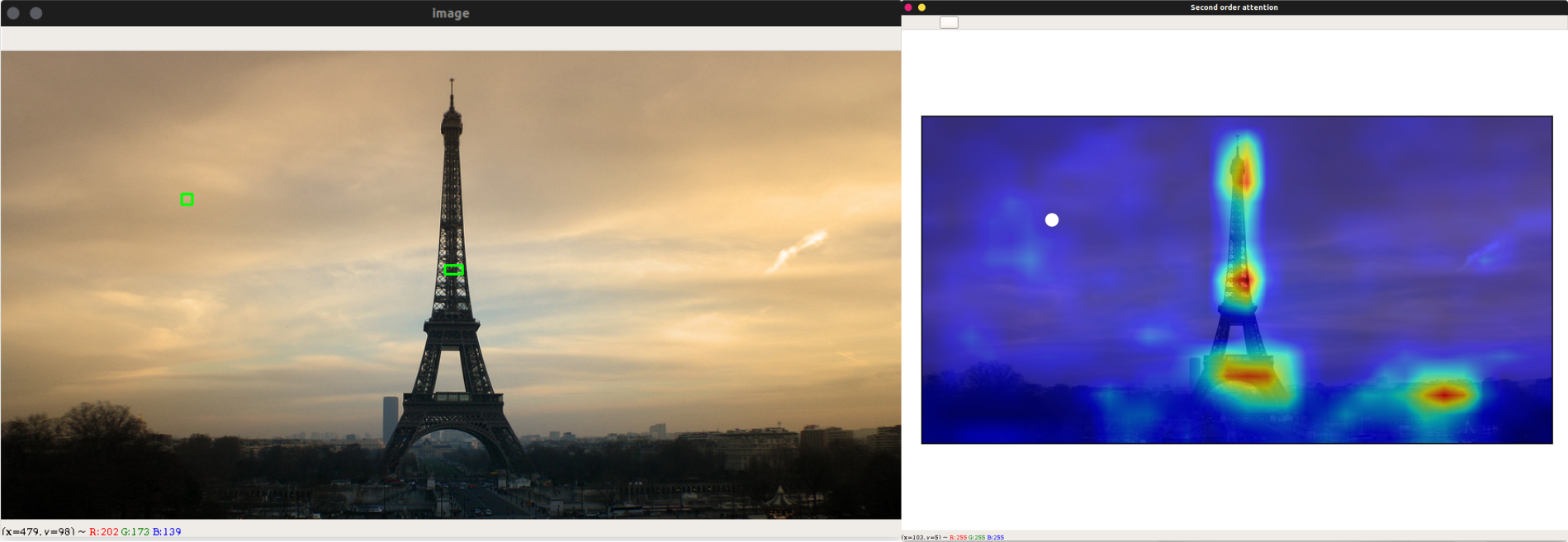
Try drawing a (light green) rectangle centred at the location you would like to visualise the SOA map
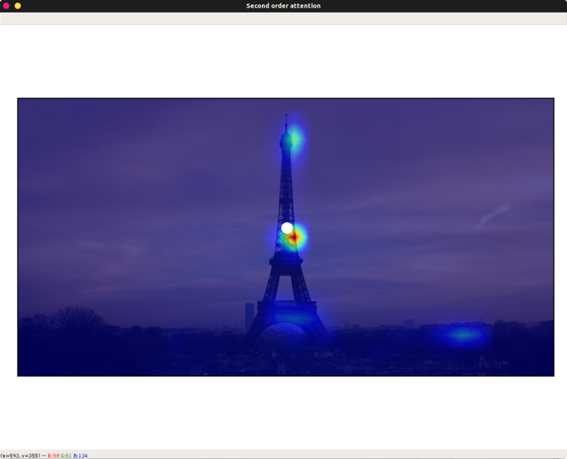
A new window titled Second order attention with the SOA from the closest location in the feature map overlaid on the image, and a white dot indicating where you've selected should appear as below
Now, try drawing a rectangle in the sky, you should see the SOA more spread-out and silhouetting the main landmarks like this
You can keep clicking around the image to visualise more SOAs. Remember, the white dot in the SOA map tells you where the currently displayed attention map is selected from!
You can also try out different images by parsing the programme with
python3 -m demo.interactive_soa --image PATH/TO/YOUR/IMAGE
Jupyter-Notebook
Coming Soon!
Simple inference
We provide a bare-bones inference code for the local counterpart of SOLAR (Section 5.3 in the paper), so you can plug it into whatever applications you have for local descriptors.
To check that it works, run
python3 -m solar_local.example
If successful, it should display the following message
SOLAR_LOCAL - SOSNet w/ SOA layers:
SOA_3:
Num channels:    in   out   mid
                 64    64    16
SOA_4:
Num channels:    in   out   mid
                 64    64    16
SOA_5:
Num channels:    in   out   mid
                128   128    64
Descriptors shape torch.Size([512, 128])
Jupyter-Notebook
Follow our demo notebook to see a comparison between solar_local and the baseline SOSNet on an image-matching toy example.
Pre-processing the training set
As the GL18 dataset consists of only URLs, many of which have already expired, this part of the code lets you download the images we had at the time of training our models. However, this also means that extra storage space would be required for extracting tarballs, so please expect to have ~700GB upwards available. Otherwise, you could still download using GL18's downloader and save the images at data/train/gl18/jpg.
To download the images and pre-process them for training, simply run
sh gl18_preprocessing.shThis would take sometime but you should then see around 1-million images in data/train/gl18/jpg and the pickle file data/train/gl18/db_gl18.pkl required for training.
If you downloaded the images from the URLs directly, please also make sure you download train.csv, boxes_split1.csv and boxes_split2.csv and save them into data/train/gl18. Then you can run
cd data/train/gl18 && python3 create_db_pickle.pyYou should then see data/train/gl18/db_gl18.pkl successfully created.
Training
Once you've downloaded and pre-processed GL18, you can start the training with the settings described in the paper by running
python3 -m solar_global.examples.train specs/gl18 --training-dataset 'gl18' --test-datasets 'roxford5k,rparis6k' --arch 'resnet101' --pool 'gem' --p 3 --loss 'triplet' --pretrained-type 'gl18' --loss-margin 1.25 --optimizer 'adam' --lr 1e-6 -ld 1e-2 --neg-num 5 --query-size 2000 --pool-size 20000 --batch-size 8 --image-size 1024 --update-every 1 --whitening --soa --soa-layers '45' --sos --lambda 10 --no-val --print-freq 10 --flatten-desc
You can monitor the training losses and image pairs with tensorboard
tensorboard --logdir specs/If you use this repository in your work, please cite our paper:
@inproceedings{ng2020solar,
    author    = {Ng, Tony and Balntas, Vassileios and Tian, Yurun and Mikolajczyk, Krystian},
    title     = {{SOLAR}: Second-Order Loss and Attention for Image Retrieval},
    booktitle = {ECCV},
    year      = {2020}
}
