This is a Julia port of the Python library pHcalc by Ryan Nelson.
As this is currently not registered, it is installed like this:
julia> using Pkg
julia> Pkg.add(url="git@github.com:tp2750/pHcalc.jl.git")The following examples are based on examples in the README from the pHcalc python package by Ryan Nelson.
The basic interface is the function acid:
acid(concentration): a strong acid as HCl, fully de-protonated at all pH. Theconcentrationis in Macid(concentration, pKa; charge=0): a weak acid given with one or more pKa values. Thechargeis the charge of the fully protonated form.acid(; concentration, pKa=missing; charge=0): all parameters can be specified as keyword parameters.
Similarly, there is a base function, which is just an alias of the acid function with pKb = 14-pKa.
See examples below.
The strong acids and bases are modeled just by the acid and base functions, where the only parameter is the molar concentration.
A solution with a concentration of 1E-2 M HCl has a pH of 2, and one with a concentration of 1E-8 M HCl has a concentration just below 7.
julia> using pHcalc
julia> pH(acid(0.01))
1.9999999999565705
julia> pH(acid(1E-8))
6.978294313542888
Similarly for NaOH:
julia> using pHcalc
julia> pH(base(1E-2))
12.00000000004343
julia> pH(base(1E-8))
7.021705686457112We model HF as an acid with pKa 3.17. First we compute the pH of 0.01 M HF, and next we titrate this with 0.01 M NaOH. Note that here we assume that we add 0.01M NaOH without changing the concentration of HF.
julia> using pHcalc
julia> HF(concentration) = acid(concentration, 3.17)
julia> pH(HF(0.01))
2.6413038913220532
julia> pH([HF(0.01), base(0.01)])
7.59919839956255Carbonic acid has 2 pKa values. The values used in by Ryan Nelson are: 6.3, 10.32. This gives:
julia> using pHcalc
julia> pH(acid(0.01, [3.6, 10.32]))
2.834379584567423
Other sources claim the pKa values to be: 6.35, 10.33 leading to a different pH value:
julia> using pHcalc
julia> pH(acid(0.01, [6.35, 10.33]))
4.176450491695669
which is consistent with the value given here.
As an example of an acid that is charged in the fully protonated form, we reproduce the Alanine Zwitterion example of the pHcalc README:
julia> using pHcalc
julia> pH(acid(0.01, [2.35, 9.69], charge=1))
6.099154517095277As a more complex example, we reproduce the ammonium phosphate example of the pHcalc README.
We used the pKa values of Phosphoric acid (H₃PO₄) are: 2.16, 7.21, 12.32, and the pKb of ammonia is 4.75.
To model 0.01 M of (NH₄)₃PO₄ we take 0.01 M of H3PO4 and 0.03 M of NH4 with a charge of +1:
julia> using pHcalc
julia> pH([acid(0.01, [2.16, 7.21, 12.32]), base(0.03, 4.75, charge=1)])
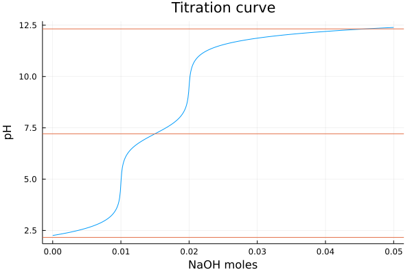
8.959447419610122We can easily plot something similar to a titration curve. However, these are not very "chemical" as it assumes we change the concentration of the base without changing the concentration of the acid. In principle this can be done with solid NaOH.
Here we use 0.01 M of phosphoric acid as example:
julia> using pHcalc
julia> using Plots
julia> function titration_curve(pKa, charge, concentration; volume = 1., base_conc =  range(1E-8, stop=.05, length=500), title="Titration curve")
           titrant = acid(concentration, pKa, charge=charge)
           tit_curve = [pH([titrant, base(x/volume)]) for x in base_conc];
           p1 = plot(base_conc, tit_curve, xlabel="NaOH moles", ylabel = "pH", label="", title=title)
           hline!(pKa, label="")
           display(p1)
       end
julia> titration_curve([2.16, 7.21, 12.32], 0., 0.01)The examples above show that we get the same values as the python library. Is it faster?
julia> using pHcalc
julia> function tit_curve(pKa, charge, concentration; volume = 1., base_conc =  range(1E-8, stop=.05, length=500))
           titrant = acid(concentration, pKa, charge=charge)
           [pH([titrant, base(x/volume)]) for x in base_conc]
       end

julia> @time c1 = tit_curve([2.16, 7.21, 12.32], 0., 0.01);
0.175207 seconds (1.10 M allocations: 47.210 MiB, 7.22% gc time)from pHcalc.pHcalc import Acid, Neutral, System
import numpy as np
import time
def tit_curve():
na_moles = np.linspace(1e-8, 5.e-2, 500)
sol_volume = 1.
phos = Acid(pKa=[2.16, 7.21, 12.32], charge=0, conc=1.e-1)
phs = []
for mol in na_moles:
na = Neutral(charge=1, conc=mol/sol_volume)
system = System(phos, na)
system.pHsolve(guess_est=True)
phs.append(system.pH)
return na_moles, phs
start_time = time.time()
x1, y1 = tit_curve()
print("--- %s seconds ---" % (time.time() - start_time))
## --- 2.083081007003784 seconds ---So the Julia version is about 12 times faster.
Does it matter? Perhaps.
We can quite acurately reproduce the pH values of Sørensen's phosphate buffer from this table using pKa values adjusted for a 100 mM ionic strength: [2.06486, 6.80506, 11.564674].
The phosphate buffer consists of a mix of the waek acid NaH2PO4 and it's conjugate base: Na2HPO4. We model these as phosphoric acid with a charge parameter given by the number of missing hydrogens:
- NaH2PO4(conc) = acid(conc, [2.065, 6.805, 11.565], charge=1)
- Na2HPO4(conc) = acid(conc, [2.065, 6.805, 11.565], charge=2)
As an example, to get a 100 mM buffer at pH 7, the table says we should mix 39.0 mM NaH2PO4 and 61.0 mM Na2HPO4. This gives:
pH([acid(0.039, [2.065, 6.805, 11.565], charge=1), acid(0.061, [2.065, 6.805, 11.565], charge=2)])
# 6.999236502941879
The recipe uses 200 mM stocks, and does a final 2X dilution. We can model that directly:
A = sample(acid(0.2, [2.065, 6.805, 11.565], charge=1), 0.039)
B = sample(acid(0.2, [2.065, 6.805, 11.565], charge=2), 0.061)
pH(dilute.(mix([A,B]),2))
# 6.999236502941879We use the same method as in Clymer / Barton to adjust for ionic strength.
In the case of phosphate, we get (at 25C):
julia> ioncorrection([2.148, 7.198, 12.375], strength=0.1)
3-element Vector{Float64}:
  2.0648590825585424
  6.805057825843171
 11.56467418465781

