Quick Zono Reach

Quickzonoreach is a python3 library for quick computations of discrete-time reach sets using zonotopes, aiming to be suitable for online computation. The system model is x' = A_i x + B_i u, where A_i and B_i can change at each step (suitable for piecewise trajectory linearized models). The initial states are given as a box and each step can have its own box input constraints and time step.

Important Functions

Important functions:

get_zonotope_reachset() (in quickzonoreach/zono.py): computes and returns the reach set, given lists for the parameters at each step.
iterate_zonotope_reachset() (in quickzonoreach/zono.py): runs a passed-in custom function on each element of the reach set, given parameters similar to get_zonotope_reachset
get_center_sim() (in quickzonoreach/sim.py): computes a center simulation using similar parameters as get_zonotope_reachset. Useful for sanity checks.
Zonotope.verts() (in quickzonoreach/zono.py): get an approximate 2-d projection of the zonotope.
Zonotope.box_bounds() (in quickzonoreach/zono.py): quick box bounds of the zonotope.
Zonotope.plot() (in quickzonoreach/zono.py): plots a 2-d projection of the zonotope with matplotlib.
Zonotope.maximize() (in quickzonoreach/zono.py): optimize over the zonotope in a given direction, for quick safety checking without LP.

Examples

Four examples are also provided:

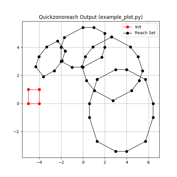
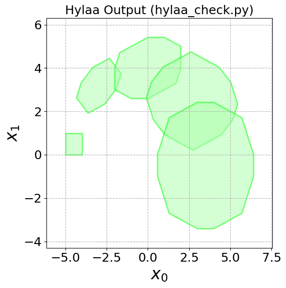
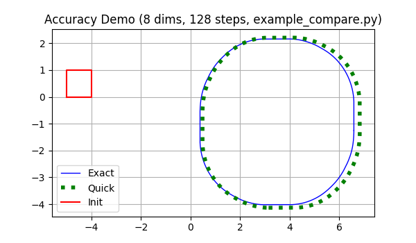
examples/example_plot.py: Produce quickzonoreach.png (the plot at the top of the README) which matches Hylaa's output, hylaa.png, that can be produced by hylaa_check.py (you'll need Hylaa installed from https://github.com/stanleybak/hylaa).
examples/example_compare.py: Compares accuracy using quick=True (Euler approximation) method vs computing full matrix exponential. The quick=True mode is fairly accurate when the time step is small. This plot is provided below.
examples/example_time_varying.py: Produces time_varying.png, which does a few steps for a medium-dimensional time-varying system, and checks that the center sim is inside the computed zonotopes.
examples/example_profile.py: Measures runtime for various step sizes and dimensions to produce the tables shown below.

Quick Matrix Exponential Mode

The quick=True parameter to get_zonotope_reachset can be used to approximate the matrix exponential by the first two terms of the series definition (e^{At} = I + At), rather than computing it with a library call to expm. This is slightly faster, and may be accurate enough especially when the time step is small. A plot showing the difference at the final time step (at time pi) for the noisy harmonic oscillator system is below:

Performance

A rough gauge of performance can be computed with example_profile.py. Performance depends in the specific system, so it may vary from when you use the library. The script will produce the tables show below.

For these measurements, we used a replicated a noisy harmonic oscillator with two inputs at each time step. The time bound is pi, and we vary the number of dimensions and time steps. The measurements are in seconds, performed on my laptop (i5-5300U CPU at 2.3GHz).

Exact Matrix Exponential, Saving All Zonotopes

Exact Save All	8 steps	16 steps	32 steps	64 steps	128 steps	256 steps
2 dims	0.08	0.08	0.2	0.3	0.6	1.2
4 dims	0.05	0.09	0.2	0.3	0.7	1.3
8 dims	0.05	0.1	0.2	0.4	0.8	1.5
16 dims	0.07	0.1	0.2	0.5	1.0	2.0
32 dims	0.1	0.2	0.3	0.7	1.4	-
64 dims	0.2	0.3	0.6	1.3	-	-
128 dims	1.0	2.0	-	-	-	-
256 dims	4.1	-	-	-	-	-

Quick Matrix Exponential, Saving All Zonotopes

Quick Save All	8 steps	16 steps	32 steps	64 steps	128 steps	256 steps	512 steps	1024 steps	2048 steps
2 dims	0.0007	0.001	0.002	0.005	0.01	0.07	0.1	0.5	1.7
4 dims	0.0005	0.0006	0.0009	0.002	0.01	0.02	0.1	0.4	1.8
8 dims	0.0004	0.0005	0.0009	0.002	0.006	0.02	0.09	0.5	1.9
16 dims	0.0005	0.0006	0.001	0.003	0.007	0.02	0.1	1.2	-
32 dims	0.002	0.003	0.005	0.008	0.01	0.06	0.3	1.5	-
64 dims	0.005	0.004	0.003	0.006	0.01	0.09	0.4	1.8	-
128 dims	0.01	0.02	0.03	0.05	0.08	0.2	0.7	2.7	-
256 dims	0.02	0.06	0.09	0.1	0.2	0.5	1.4	-	-
512 dims	0.1	0.2	0.3	0.5	0.9	1.8	-	-	-
1024 dims	0.5	0.7	1.1	-	-	-	-	-	-
2048 dims	2.3	-	-	-	-	-	-	-	-

Quick Matrix Exponential, Saving Only the Last Zonotope

Which zonotopes are saved can be controlled with the save_list parameter to get_zonotope_reachset. If you're doing many steps or working in high dimensions, saving copies at every step can sometimes slow things down.

Quick Save Last	32 steps	64 steps	128 steps	256 steps	512 steps	1024 steps	2048 steps	4096 steps	8192 steps	16384 steps	32768 steps
2 dims	0.002	0.003	0.006	0.02	0.02	0.04	0.04	0.1	0.3	1.0	3.3
4 dims	0.0006	0.0009	0.002	0.004	0.008	0.02	0.05	0.2	0.5	2.8	-
8 dims	0.002	0.003	0.006	0.02	0.03	0.03	0.08	0.5	1.8	-	-
16 dims	0.002	0.004	0.008	0.02	0.05	0.1	0.3	0.9	3.2	-	-
32 dims	0.004	0.006	0.02	0.03	0.08	0.2	0.6	2.0	-	-	-
64 dims	0.008	0.01	0.02	0.05	0.1	0.3	1.1	-	-	-	-
128 dims	0.06	0.04	0.06	0.1	0.3	0.8	3.4	-	-	-	-
256 dims	0.1	0.1	0.2	0.4	1.0	3.0	-	-	-	-	-
512 dims	0.3	0.4	0.7	1.5	-	-	-	-	-	-	-
1024 dims	1.2	-	-	-	-	-	-	-	-	-	-

Docker Container & Continous Integration

There exists a Docker container which in theory should make sure the examples can execute after each commit, as indicated by the image at the top of the README. For details, see the commands and comments in the Dockerfile. To run the examples in Docker do:

docker build -t quickzonoreach .
docker run quickzonoreach

Ideas for More Speed

If using quick and only saving some of the zonotopes is still too slow, make sure you have a good version of BLAS installed like OpenBlas (matrix dot product in numpy is an important operation for speed). It may be possible to use 32-bit floats instead of 64 bit.

Also, the library is currently single-threaded, so using multiple cores or GPUs for computation could increase speed more, although this would need code modification.

trhoangdung/quickzonoreach