Machine Learning Models
This repo contains a variety of machine learning models built from scratch (using just pure mathematics & without any built-in machine learning capabilities from libraries). All of the models were built using Python + Numpy + math and visualized with Matplotlib. This repo also includes a full explanation behind the mathematics of each model along with how to use each script.
Included Models
- (Gradient Descent) Uni/Multi-Variate Linear Regression
- (Gradient Descent) Uni/Multi-Variate Quadratic Regression
- (Normal Equation) Uni/Multi-Variate Linear Regression
- (Normal Equation) Uni/Multi-Variate Quadratic Regression
- Currently working on Univariate Sinusoidal Regressions, Logistic Regressions, & Neural Networks. Repo will be updated once those are finalized!
Notes
- Python 3.10+ w/ Tkinter is required.
- Make sure all dependencies are installed before running any of the scripts.
pip3 install -r requirements.txt
- Prerequisite knowledge (to understand the mathematics behind each model):
- Multivariable calculus.
- Linear algebra.
- All inputs will be CSV files that meet the following requirements:
- All rows have the same number of columns.
- Contains only numeric values.
- Values are separated by commas.
- No trailing commas.
- Has at least two lines.
- The last line contains the y-values.
- All previous lines contain the x-values.
(Gradient Descent) Uni/Multi-Variate Linear Regression
Let's briefly cover some standard notation:
-
$\vec{x}$ : input vector (feature). -
$\vec{y}$ : output vector (label). -
$\hat{y}$ : predicted output. -
$m$ : number of training examples. -
$n$ : number of input variables. -
$(x^{(i)}, y^{(i)})$ :$i^{th}$ training example.
Univariate case: let's say we have the following table of experimental data:
| x | y |
|---|---|
| -10 | 26 |
| -10 | 28 |
| -9 | 22 |
| -8 | 22 |
| -7 | 14 |
| -6 | 15 |
| -5 | 11 |
| -4 | 12 |
| -4 | 10 |
| -3 | 9 |
| -2 | 6 |
| -1 | 3 |
| 0 | -1 |
| 0 | 1 |
| 1 | -0 |
| 2 | -5 |
| 3 | -4 |
| 4 | -10 |
| 5 | -10 |
Our goal is to predict how
We want to continually adjust our weights, so that our cost decreases over time. In order to do this, we must calculate how much each weight is contributing towards the cost (this is called the gradient). This is given by the following partial derivatives (given in scalar and vector/matrix versions):
Now all we need to do is repeat the following operations until our algorithm converges (again, both scalar and matrix versions):
Note that these updates must be done simultaneously. Also, src/data/gradient/linear/univariate.csv):
-10, -10, -9, -8, -7, -6, -5, -4, -4, -3, -2, -1,  0, 0, 1,  2,  3,   4,   5
 26,  28, 22, 22, 14, 15, 11, 12, 10,  9,  6,  3, -1, 1, 0, -5, -4, -10, -10
Navigate to the src directory and find the config.json file. Make the following changes if necessary:
{
    "regression_method": "gradient",
    "regression_type": "linear",
    "input_file_path": "data/normal/linear/univariate.csv"
}
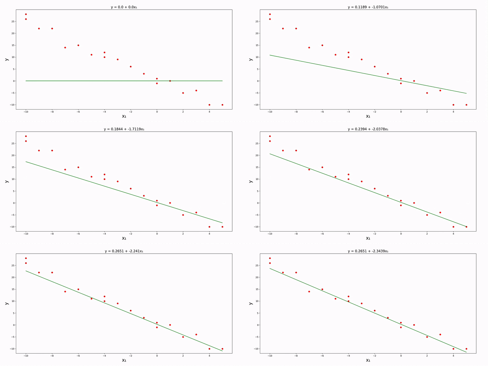
The parameter_precision key can be optionally modified (in this example, it's set to 4). After running main.py, we can see the plot of our data along with the linear regression line:
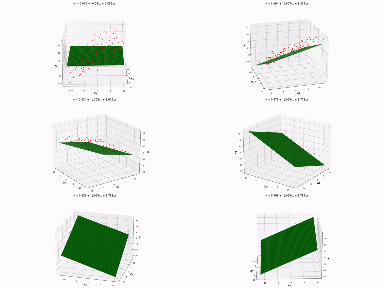
Bivariate case: the math works out similarly with two inputs as well. Let's try to see how the experimental data found in src/data/linear/bivariate can be modeled. We'll need to slightly modify our config.json file beforehand:
{
    "regression_method": "gradient",
    "regression_type": "linear",
    "input_file_path": "data/normal/linear/bivariate.csv"
}
Running main.py yields:
Trivariate case: modify config.json so that it matches the following:
{
    "regression_method": "gradient",
    "regression_type": "linear",
    "input_file_path": "data/normal/linear/trivariate.csv"
}
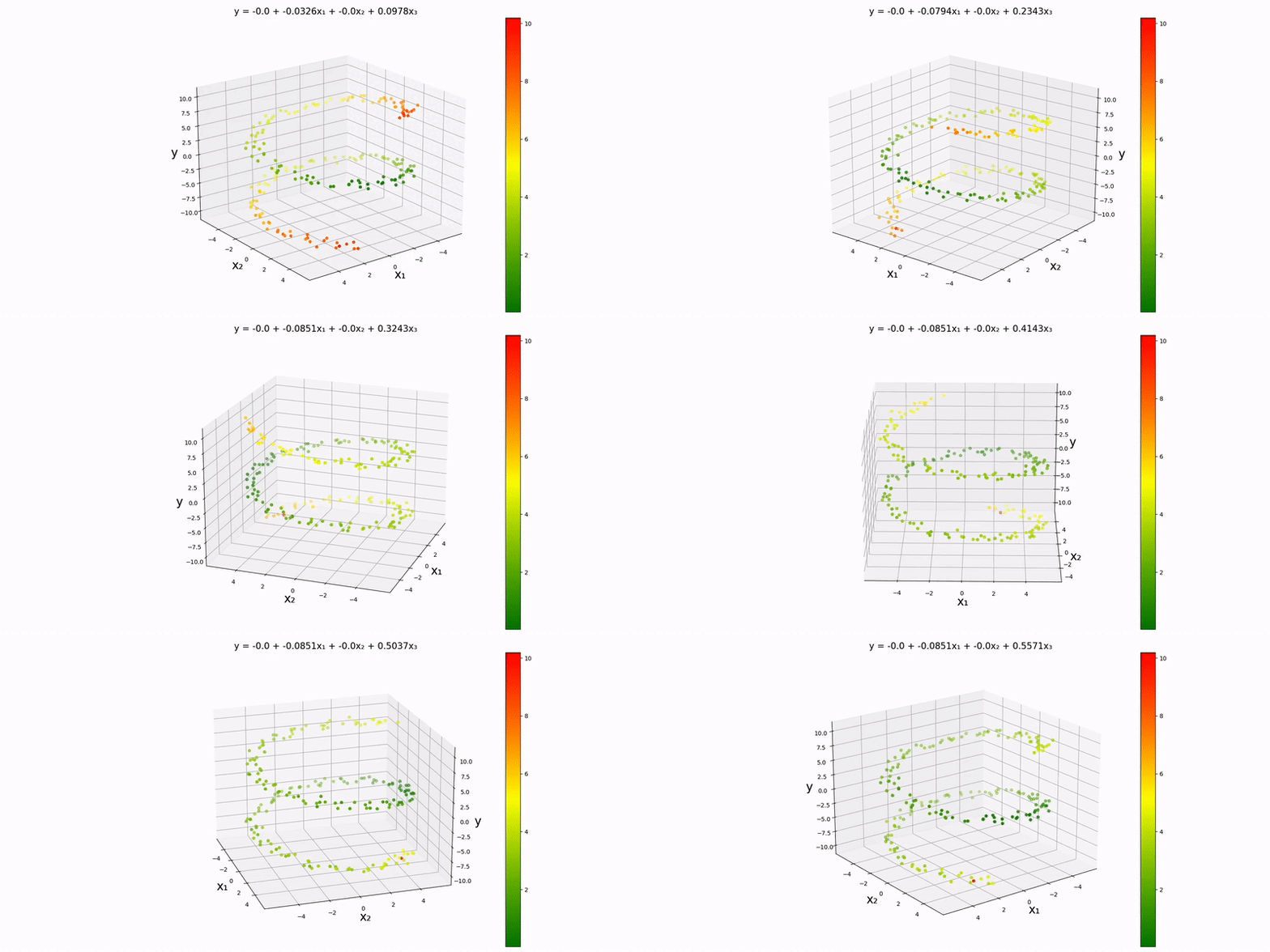
Run main.py to visualize:
This is basically a contour map but in one higher dimension. The colors represent how bad our prediction is. Over time, we can see that everything slowly starts turning green as our weights improve. Note that there is one tiny datapoint that stays stagnant throughout; this is purposefully done, so we can see how the colors change as training progresses.
Multivariate with more than 3 inputs: visualization will be near impossible. The script will continually produce multiple outputs similar to like this instead:
y = 20.0 + 16.96(x_1) + 20.58(x_2) + 16.96(x_3) + 20.58(x_4)
(Gradient Descent) Uni/Multi-Variate Quadratic Regression
Quadratic regressions are very similar to linear regressions.
Univariate case: use following parameter vector and design matrix (hypothesis function stays the same):
The math magically works out because of the way we used vectors/matrices to set things up. Let's use the following configurations for our config.json file:
{
    "regression_method": "gradient",
    "regression_type": "quadratic",
    "input_file_path": "data/gradient/quadratic/univariate.csv",
}
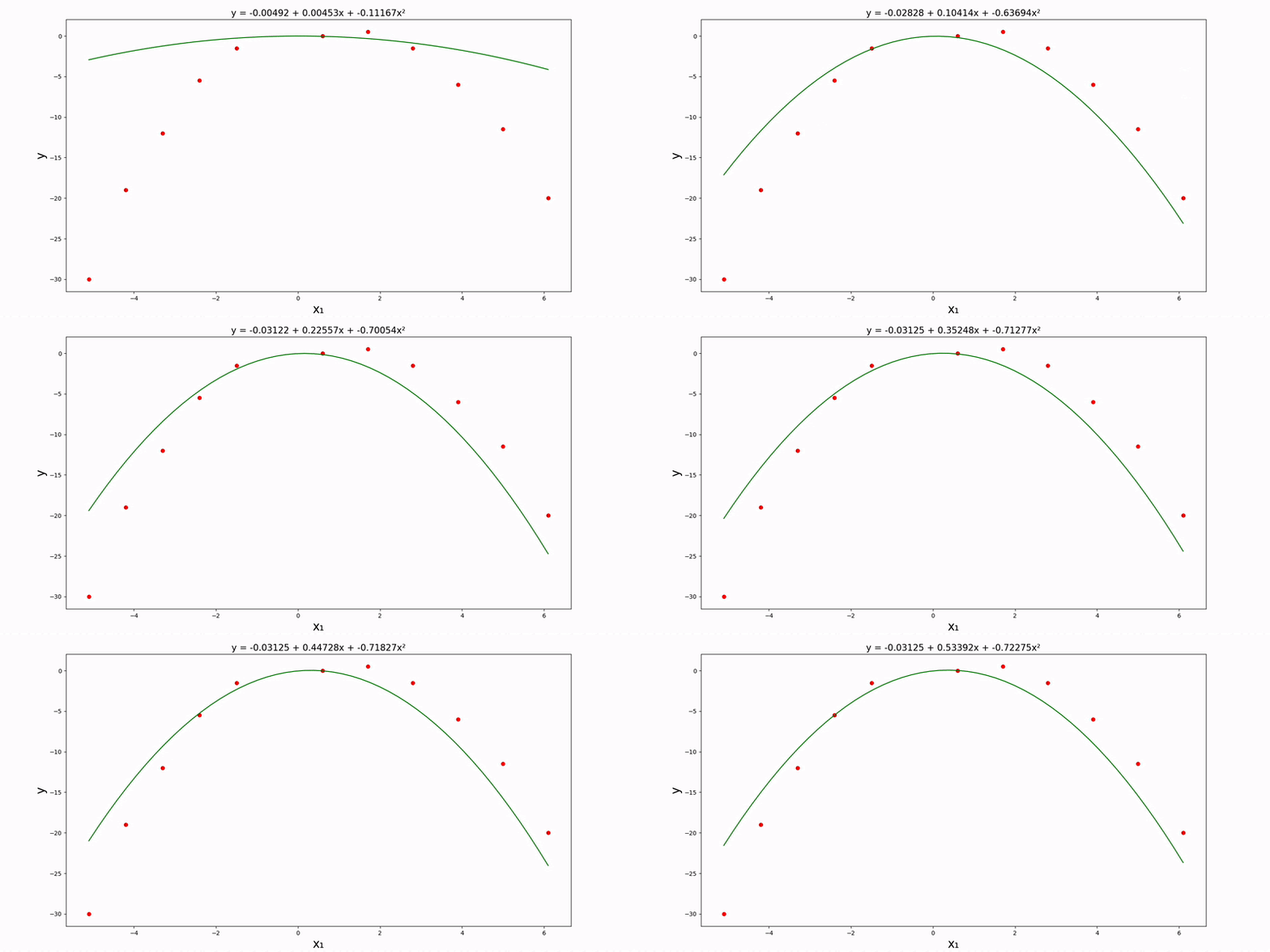
Running script.py outputs:
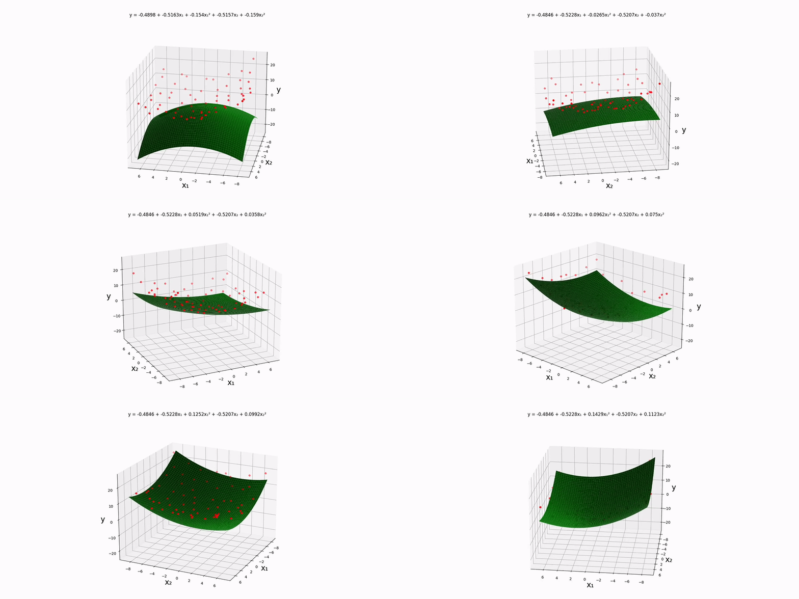
Bivariate case: similar to the univariate case, we can set things up for the bivariate case like so:
Setting up config.json:
{
    "regression_method": "gradient",
    "regression_type": "quadratic",
    "input_file_path": "data/gradient/quadratic/bivariate.csv",
}
Running script.py:
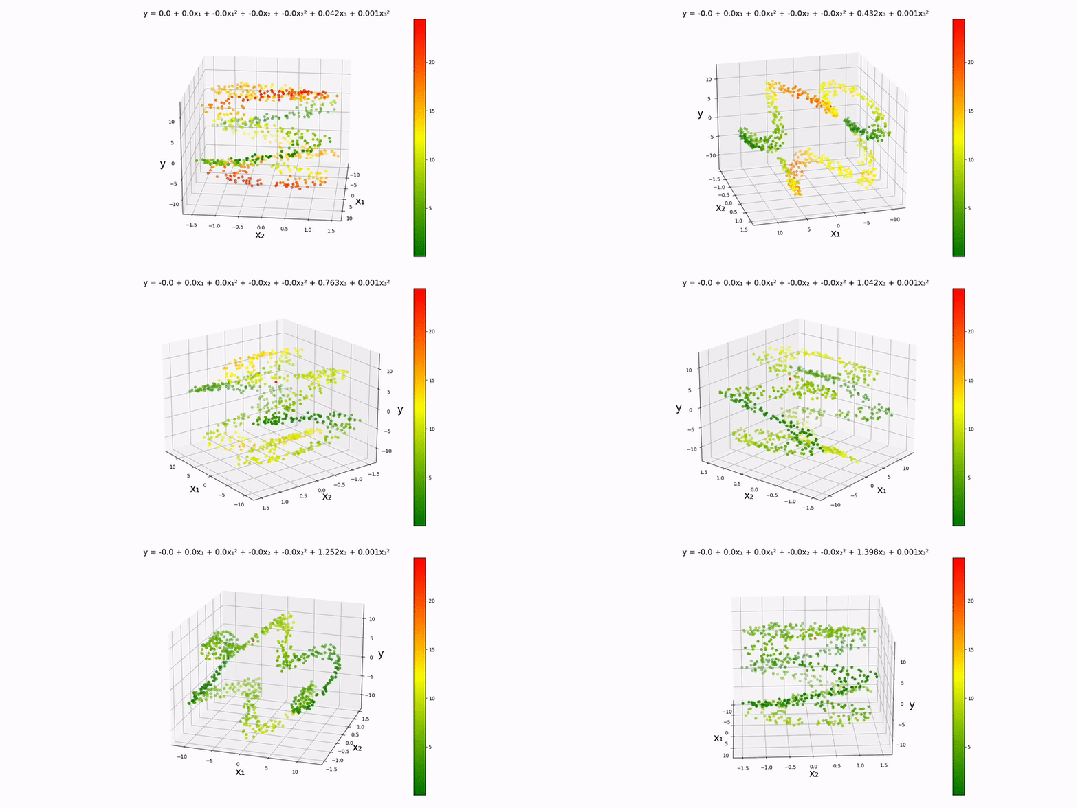
Trivariate case: hopefully we can spot the pattern for how to set up the parameter vector and design matrix by now:
Setting up config.json:
{
    "regression_method": "gradient",
    "regression_type": "quadratic",
    "input_file_path": "data/gradient/quadratic/trivariate.csv",
}
Running script.py:
Like with the trivariate linear regression, I should mention that this is essentially a contour map in one higher dimension with the colors representing how bad our prediction is. The dots slowly turn green as training progresses. And again, there is one tiny datapoint that stays stagnant throughout; this is purposefully done, so we can see how the colors change over time.
Multivariate with more than 3 inputs: visualization will be difficult. Instead, the script will continually produce multiple outputs similar to like this:
y = 0.0 + 0.0(x_1) + 0.0(x_1)² + -0.0(x_2) + 0.0(x_2)² + 0.3901(x_3) + 0.017(x_3)² + 0.7933(x_4) + -0.0042(x_4)²
(Normal Equation) Uni/Multi-Variate Linear Regression
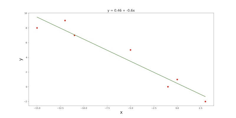
Univariate case: after exploring a single-variable regression first, we'll have a look at multi-variable regressions afterwards. Let's say we have the following experimental data, and we want to find the line of best fit to make predictions for other inputs.
| x | y |
|---|---|
| -15 | 8 |
| -12 | 9 |
| -11 | 7 |
| -5 | 5 |
| -1 | 0 |
| 0 | 1 |
| 3 | -2 |
Suppose each
Let
The third line is called the normal equation. Calculating src/data/normal/linear/univariate.csv):
-15, -12, -11, -5, -1, 0,  3
  8,   9,   7,  5,  0, 1, -2
Next, navigate to the src directory, and find the config.json file. Make sure the value of regression_method on line 2 is set to "normal", regression_type on line 3 is set to "linear", and input_file_path on line 3 is set to "data/normal/linear/univariate.csv". We may optionally modify parameter_precision on line 5 to change the amount of decimals our main.py, the output should look something like this:
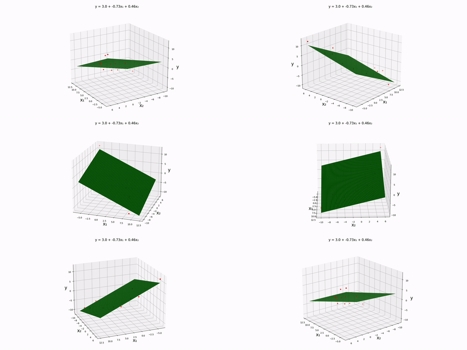
Bivariate case: our design matrix's left-most column should still contain all ones, but this time, the subsequent columns should contain the input data points. Notice that src/data/normal/linear/bivariate.csv):
| x₁ | x₂ | y |
|---|---|---|
| -6 | 6 | 12 |
| 0 | 5 | 4 |
| 1 | 3 | 7 |
| 2 | 4 | 3 |
| 4 | 2 | -2 |
| 5 | -1 | -4 |
| 7 | -4 | -6 |
| 11 | -4 | -5 |
| 8 | -7 | -4 |
| 12 | -6 | -6 |
| 9 | -10 | -10 |
-6,  0, 1, 2,  4,  5,  7, 11,  8, 12,   9
 6,  5, 3, 4,  2, -1, -4, -4, -7, -6, -10
 12, 4, 7, 3, -2, -4, -6, -5, -4, -6, -10
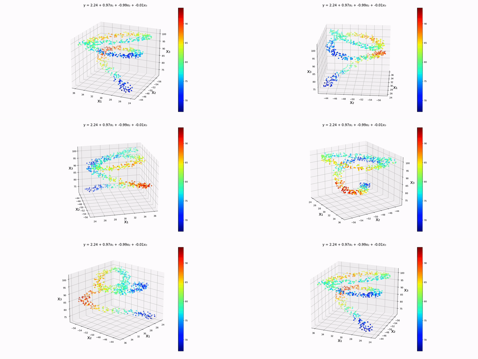
The first, second, and third lines represent the data points for config.json file so that input_file_path is set to "src/data/normal/linear/bivariate.csv". Running the main.py yields the plane of best fit for our dataset:
Trivariate case: using "src/data/normal/linear/trivariate.csv" as our input file, we can see that a decent approximation for this dataset would be
This makes sense because it seems like the plane
Multivariate with more than 3 inputs: this idea can be extended to higher dimensions as well. Although no plot would be generated, the script still produces an output in this format:
y = -1.43 + 1.03(x_1) + 0.24(x_2) + 0.39(x_3) + 0.32(x_4)
(Normal Equation) Uni/Multi-Variate Quadratic Regression
With quadratic regressions, the math works out almost identically to linear regressions.
Univariate case:
Double-cheeck that we're still in the src directory. Let's modify config.json so that the value of regression_method is "normal", regression_type is "quadratic", and input_file_path is "data/normal/quadratic/univariate.csv". Here is what it looks like:
0,  1, 2, 3, 4, 5, 6, 7,  8,  9
8, 10, 6, 4, 6, 5, 7, 9, 12, 13
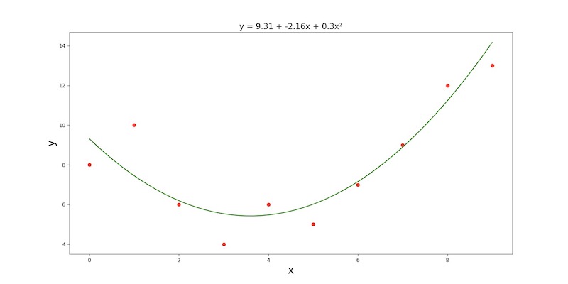
After running main.py, we get the following plot and quadratic regression equation:
Bivariate case:
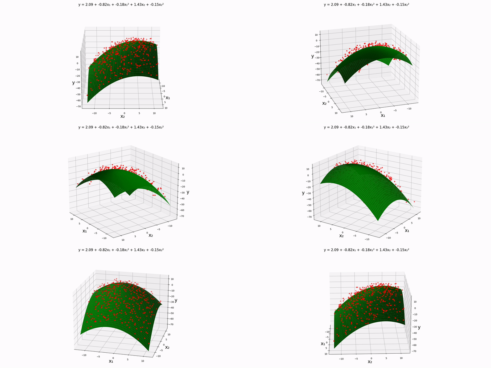
Using the example experimental data in data/normal/quadratic/bivariate.csv (and changing config.json accordingly), we get the following output:
Trivariate case: as you can probably guess, our design matrix will look something like:
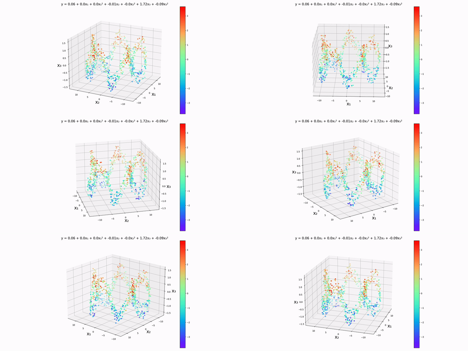
Again, we'll be using an analog of a contour map in one higher dimension to visualize this. Using the example datapoints in data/normal/quadratic/trivariate.csv (and changing config.json accordingly), we get the following output:
Just by looking at the output, the y-values to seem to depend almost exclusively on
Polynomial regressions of higher degrees or with more inputs: the same idea can be applied as long as the design matrix is set up properly and the normal equation is used, but it will be tough to visualize! Here is an output output using 4 input variables:
y = 0.06 + 0.01(x_1) + 0.10(x_1)² + -0.27(x_2) + -0.09(x_2)² + -0.84(x_3) + -0.32(x_3)² + 1.08(x_4) + -2.055(x_4)²
