The Main public server of the Galaxy Project (https://usegalaxy.org) has been collecting extensive job run data on all analyses since 2013. This large collection of job runs with attributes can be leveraged to determine more efficient ways for allocation of server resources. In addition, these data represent the largest, most comprehensive dataset available to date on the runtime dynamics for some of the most popular biological data analysis software. In this work we were aiming at creating a model to predict the runtime and maximum memory usage of complex algorithms trained on real data. In this paper we will:
- Present statistical summaries of the dataset, describe its structure, identify the presence of undetected errors, and discuss any other insights into the Galaxy server that we believe will be useful to the community.
- Confirm that the random forest regressor gives the best performance for predicting the runtime of complex algorithms as was seen by Hutter et al.
- Discuss the benefits and drawbacks of using a quantile random forest for creating runtime prediction confidence intervals.
- Consider the applicability of runtime and memory use prediction for tools run on Galaxy servers with different hardware.
Studying the Galaxy Project dataset reveals that there may be room to fine tune the resource allocation. The ability to determine appropriate walltimes and RAM allowance will save server resources from jobs that result in errors undetected by the server. Once freed, these resources can then be used to reduce queue wait times and increase volume of jobs processed by the server.
- Background
- Overview of Data
- Model Comparison
- Estimating a Range of Runtimes
- Using a random forest classifier
- Maximum Memory use Prediction
- Walltime and Memory Requirement Estimations as an API
- Future Work
- References
The Galaxy Project is a platform that allows researchers to run popular bioinformatics analyses on designated servers. Running a popular analysis requires downloading, configuring, and troubleshooting the analysis software on one's own machines. This can be a difficult and time consuming task.
With the Galaxy Project, researchers can run analyses using the graphical user interface through the web. To do so, the user needs only to connect to a Galaxy server (e.g. https://www.usegalaxy.org), upload their data, choose the analysis and the analysis parameters, and hit run.
The Galaxy Project has been storing the information about the execution of these analyses since 2013, and, to date, has the largest dataset of the performance of popular bioinformatics tools. We begin to study this dataset in this paper.
For more information visit https://www.galaxyproject.org.
All Galaxy instances have an option to keep records of runtime data. This is a service that adminstrators can select when configuring a Galaxy. The most widely used Galaxy instance, Galaxy main, does so, and the data collected on Galaxy main is the data used in these tests.
If adminstrators of other Galaxy instances would like to share their runtime data with the community, they can do so with the Galactic Radio Telescope (GRT). The GRT is an API service that allows Galaxy admins to export their data and have it released to the public in a standard package. For more information visit the documentation.
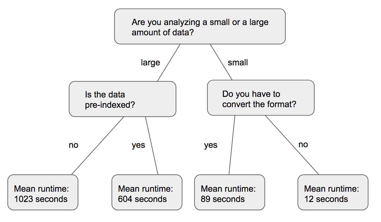
A random forest is a collection of decision trees which themselves are series of questions asked about an object. At the end of the questions, a previously unknown attribute of the object is guessed. An example of a decision tree is shown below. In this case, the decision tree tries predicting how long a job is going to take.
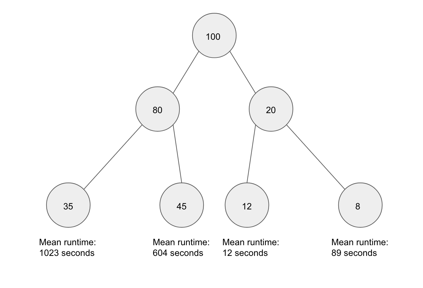
The decision tree learns what questions to ask by training on a set of previous jobs. At each node, it looks at a subset of attributes and chooses to split the data in the way that minimizes variability in the subsequent two nodes. In this way, it sorts objects by similarity of the dependent and independent variables. In the figure below, a decision tree is training on a set of 100 jobs. All 100 jobs start at the root node, and they are split up as they travel down the tree. Once the tree is trained, it can then be used to predict the runtime of previously unseen jobs.
A random forest is a collection of decision trees, each of which are trained with a unique random seed. The random seed determines which sub-sample of the data each decision tree is trained and which sub-sample of attributes each tree uses and which splits each tree attempts. By implementing these constraints, the random forest protects itself from overfitting - a problem to which decision trees are susceptible.
Incidentally, the decision tree also offers a way to see which independent attributes have the greatest effect on the dependent attribute. The more often a decision tree uses an attribute to split a node, the larger its implied effect on the dependent attribute. The scikit-learn Random Forest classes have a way of retrieving this information with the feature_importances_ class attribute.
The prediction of runtimes of complex algorithms using machine learning approaches has been done before. [1][2][3][4][5]
The popularity of cloud computing has also stimulated activity in the problem of resource usage prediction. [6][7][8] The methods developed for cloud computing, however, typically scale virtual machines with no knowledge of the programs or algorithms are being run. The predictions are based on traffic and usage patterns at seqential time steps. Since we are not interested in predicting resource usage based on time usage patterns, we forego these methods.
In a few works, new machine learning methods are designed specifically to estimate a complex algorithms' resource requirements. In 2008, Gupta et al. proposed a tool called a PQR (Predicting Query Runtime) Tree to classify the runtime of queries that users place on a server. The PQR tree dynamically choose runtime bins during training that would be appropriate for a set of historical query runtimes. The paper notes that the PQR Tree outperforms the decision tree.
Most previous works tweak and tailor old machine learning methods to the problem. For instance, in 2010, Matsunaga enhances on the PQR Tree by adding linear regressors at its leaves, naming it PQR2. They test their model against two bioinformatic analyses tools: BLAST (a local alignment algorithm) and RAxML (a phylogenetic tree constructer). The downside of PQR2 is that there are not readily available libraries of the model in popular programming languages like Python or R.
The most comprehensive survey of runtime prediction models was done by Hutter et al. In 2014. In the paper, they compared 11 regressors including ridge regression, neural networks, Gaussian process regression, and random forests. They did not include PQR tree in their evaluations. They found that the random forest outperforms the other regressors in nearly all runtime prediction assessments and is able to handle high dimensional data without the need of feature selection.
In our paper, we verify that random forests are the best model for the regression, adding two popular ensemble methods to the comparison. We consider the use of quantile regression and classification for walltime and maximum memory usage estimation. Finally, we discuss [dicuss -> test once we get euro data] the plausibility of an API that provides resource use estimation for Galaxy jobs.
All of the tool executions on https://usegalaxy.org are tracked, and a comprehensive set of job run attributes are recorded.
This includes:
Job Info
- id
- user_id
- tool_id
- tool_version
- state
- create_time
Numeric Metrics
- processor_count
- memtotal
- swaptotal
- runtime_seconds
- galaxy_slots
- start_epoch
- end_epoch
- galaxy_memory_mb
- memory.oom_control.under_oom
- memory.oom_control.oom_kill_disable
- cpuacct.usage
- memory.max_usage_in_bytes
- memory.memsw.max_usage_in_bytes
- memory.failcnt
- memory.memsw.limit_in_bytes
- memory.limit_in_bytes
- memory.soft_limit_in_bytes
User Selected Parameters
- tool specific
Datasets
- sizes of input and output files
- extensions of input and output files
The Galaxy Main dataset contains runtime data for 1371 different tools that were run on the Galaxy Servers over the past five years. A statistical summary of those tools, ordered by most popular, can be found at summary_statistics.csv. The runtimes are in seconds. The full dataset of jobs run on Galaxy Main can be found at https://telescope.galaxyproject.org. The telescope webpage also hosts datasets of jobs run on other Galaxy instances, such as Galaxy Europe.
The versions listed are the version of the Galaxy wrapper of the tool, not the version of the underlying tool itself. Galaxy Main has three server clusters to which it sends jobs. The clusters have different hardware specifications, and the clusters themselves may exhibit heterogeneous configurations. Because the jobs are run on a remote site, the Galaxy Main instance does not know which hardware is assigned to which job. In addition, The CPUs of the nodes are shared with other jobs running concurrently, so the performance of jobs is also effected by the server load at the time of execution. These attributes are not in the published dataset because of the difficulty of tracking them.
Typically, machine learning algorithms, such as, random forests and neural networks prefer to use data with a normal distribution. The distribution of runtimes and file sizes in the Galaxy dataset are highly skewed. The distribution for a tool called BWA (Galaxy version 0.7.15.1) can be seen below.
In this project, we address this skewness by doing a log transform on the data. We use numpy's log transformer numpy.log1p which transforms the data by log(1+x)
This transformation works for most of the runtime and input file size attributes to give a more balanced distribution.
A hurdle the dataset presents is that it contains undetected errors - errors that occurred but were not recorded.
One type of undetected error is the input file error, in which jobs are recorded to have completed 'succefully' without the requisite input data. For instance, there are 49 jobs of the tool bwa_mem Galaxy version 0.7.15.1 (link) that completed succesfully without the requisite input. This comprises .25% of 'successful' jobs recorded for this tool.
Whether these errors are caused by bugs in the tool code, malfunctions in the server, mistakes in record keeping, or a combination of these, the presence of these of errors casts doubt on the validity of the rest of the dataset. If there are many jobs similarly mislabelled as "successfully completed" that are not as easily identified as input file errors, it will bias the predictions and the performance metrics, which are computed on the same, possibly contaminated, dataset.
One method of screening the dataset is by excluding extreme values.
This requires choosing quantiles of contamination for each tool. This method may exclude a portion of the bad jobs, but it does not exclude them all and will also exclude good jobs.
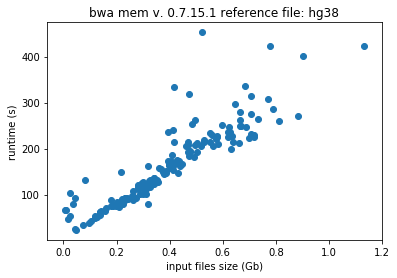
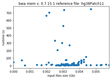
Take the following example. Freeze all the user selected parameters, except for input file size. We can freeze the reference file size because many reference genomes, such as the human genome, are popular and commonly used. The runtimes, therefore, should be directly proportional to the input file sizes. This result of this procedure can be seen in the following two plots.
User selected parameters are frozen in the above plot, and the reference file, hg38 and hg38Patch11 are two versions of the human genome. In the plot to the left, the relation between runtime and input file size is as expected. In the plot to the right, there appears to be no correlation between the two attributes. By trimming the dataset and excluding the most extreme values, only a portion of the bad jobs are addressed.
Manually finding and removing bad jobs from the dataset is the most likely the best method for cleaning it. However, this is time consuming as it requires examining each tool individually or, at the least, it requires writing instructions for each tool individually - instructions that the computer can follow to do the pruning.
A final method of undetected error detection that we will discuss is with the use of an isolation forest. In a regular random forest, a node in a decision tree chooses to divide data based on the attribute and split that most greatly decreases that variability of the following to datasets. In an isolation forest, the data is split based on a random selection of an attribute and split. The longer it takes to isolate a datapoint, the less likely it is an outlier. As with removing the tails of the runtime distribution, we need to choose the percentage of jobs that are bad before hand.
To remove bad jobs, we used the isolation forest with contamination=0.05. We also removed any obvious undetected errors, such as no-input-file errors, wherever we could.
Galaxy records all parameters passed through the command line. This presents in the dataset as a mixed bag of relevant and irrelevant attributes. A brief sample follows:
| Relevant attributes | Irrelevant attributes |
|---|---|
| file sizes | labels (such as plot axes names) |
| indexing information | redundant parameters (two attributes that represent the same information) |
| algorithm parameters selection | identification numbers (such as file ids) |
For a few, popular tools, we manually select which parameters to use. However, since we have many tools, with incongruous naming schemes and unique parameters, we cannot do this for each tool. Instead, we created a heuristic to eliminate common irrelevant features. The simple heuristic attempts to remove any labels or identification numbers that are present. Although it does not search for redundant parameters, it can be altered to do so.
The parameters are screened in the following way:
- Remove likely irrelevant parameters such as:
- workflow_invocation_uuid
- chromInfo
- parameters whose name begins with
- __job_resource
- rg (i.e. read groups)
- reference_source (this is often redundant to dbkey)
- parameters whose names end with
- id
- indeces
- identifier
- Remove any non-numerical parameter whose number of unique values exceeds a threshold
- Remove parameters whose number of undecalared insatances exceed a threshold
- Remove parameters that are list or dict representations of objects
With these filters, we are able to remove computationally costly parameters. Since identifiers and labels are more likely to explode in size when binarized and dilute the importance of other attirbutes, we are most concerned with removing those. In this paper, we used a unique category threshold of 100 and a undeclared instance threshold of 0.75 * number of instances.
As previously noted, if a continuous variables is highly skewed, it is log transformed with numpy.log1p. All continuous variables are scaled to the range [0,1] with sklearn.preprocessing.MinMaxScaler.
Categorical variables are binarized using sklearn.preprocessing.LabelBinarizer. An example of label binarization is shown below. The categorical variable 'analysis_type' is expanded into four discrete variables that can take the value 0 or 1.
| x1 | x2 | x3 | x4 | |
|---|---|---|---|---|
| illumina | 1 | 0 | 0 | 0 |
| full | 0 | 1 | 0 | 0 |
| pacbio | 0 | 0 | 1 | 0 |
| ont2d | 0 | 0 | 0 | 1 |
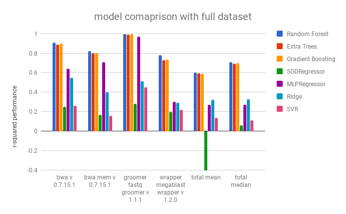
In this work, we trained popular regression models available on scikit-learn and compared their performance. We used a cross validation of three and tested the models on the dataset of each tool without the exclusion any undedected errors and with the exclusion of undetected errors via the isolation forest with contamination=5%, and compared the performance of the regressors with using the r-squared score metric. As you will see, pruning the datasets with the isolation forest improved the performance of some of the regressors, but it did not improve the performance of the random forest regressor.
For most of the tools, we used the default settings provided by sklearn library: SVR, Ridge Regressor, SGD Regressor, and Gradient Boosting regressor. The neural network (sklearn.neural_network.MLPRegressor) had two hidden layers of sizes [100,10] with the rest of the attributes set to default, and the random forest and extra trees regressors had 100 estimators and a max_depth of 12.
The table below shows the r-squared score for a select number of tools. The total mean and median were taken as the performance of the tool over every tool with more than 100 recorded runs.
The Random Forest, the Extra Treest Regressor, and the Gradient Boosting Regressor have compariable performances, but the Random Forest performs slightly better. They are followed by the feed forward neural network (MLPRegressor). It seems that many of the regressors are unable to handle the high dimensional, and mixed continuous/categorical, dataset.
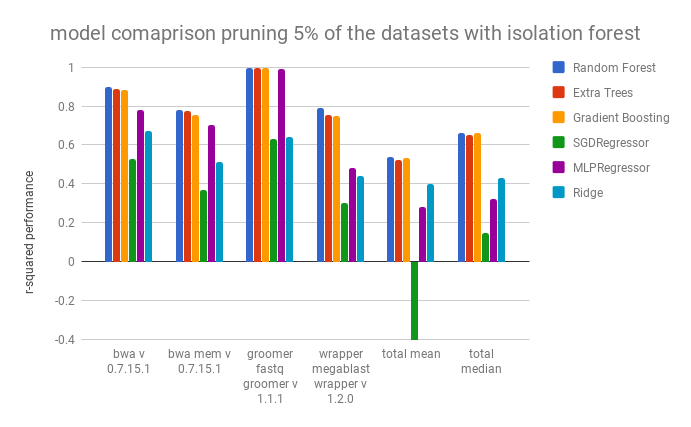
Pruning out outliers with contamination=0.05 affected the predictions as follows. SVR Regression was not performed in these tests because of the length of time required to comlete them.
Pruning the outliers with the isolation forest improved the performance of the MLPRegressor, the Ridge Regressor, and the SGD Regressor. Surpisingly, it did not improve the performance of the Random Forest Regressor or Extra Trees. Because of this, we did not continue to use the dataset pruned by the isolation forest for the remainder of the tests.
The full results can be viewed benchmarks/comparison_benchmarks.csv. It includes the time (in seconds) to train the model. The performance is marked as NaN if it's r-squared scores was below -1000.0, as was often the case with the linear regressor. We also marked a score as NaN if a model took more than 5 minutes to train, as was sometimes the case with the SVR Regressor, whose complexity scales quickly with the size of the training set. And the results for the dataset pruned with the isolation forest can be found at benchmarks/comparison_benchmarks_minus_outliers.csv. The results can be replicated with scripts/comparison_benchmarks.py
The random forest gave us the best results for estimating the runtime of a job. It would also be of interest to calculate a confidence interval for the runtime of a job. This way, when using the model to choose walltimes, we lower the risk of ending jobs prematurely.
A quantile regression forest can be used for such a purpose. A quantile forest works similarly to a normal random forest, except that at the leaves of its trees, the quantile random forest not only stores the means of the variable to predict, but all of the values found in the training set. By doing this, it allows us to calculate a confidence interval for the runtime of a job based on similar jobs that have been run in the past.
However, storing the entire dataset in the leaves of every tree is computationally costly. An alternative method is to store only the means and the standard deviations. Doing so reduces the precision of the confidence interval, but saves space. We used the modified version of the quantile regression forest that is described in Hutter et al. that uses standard deviation instead of quantiles.
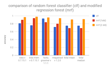
We tested the modified regression forest against the historical data with three fold validation on the full dataset. The accuracy was recorded as a prediction that is within one, two, or three standard deviations of the actual value. Because we are calculating standard deviations in these tests, we did not normalize the runtime distribution with a log transformation.
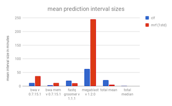
The largest drawback of the quantile regression forest is that there is no control over the time ranges that are produced and the confidence intervals can be quite large. These large time ranges may not be useful for giving a user an idea of how long an analysis will take, but they may be useful for creating walltimes.
The confidence intervals for one standard deviation are larger than those found previously, which accounts for the better accuracy at that grade. The intervals can still be quite large. The mean interval for bwa for one st. dev. is about 2000 seconds, over half an hour. Depending on the use case, this may be reasonable. To replicate these results use scripts/modified_random_forest_metrics.py
The main advantage of a random forest classifier over a quantile regression forest (or a modified regression forest using standard deviations), is that you can select the sizes of the runtime bins. Where in the quantile regression forest, you are at the mercy of the bins dynamically selected by the model.
In our tests, we chose buckets in the following manner.
- We ordered the jobs by length of runtime.
- Then, we made (0, median] our first bucket.
- We recursively took the median of the remaining runtimes until the number of remaining bucket held less than 100 instances.
|------------50%-----------|-----25%-----|--12.5%--|--12.5%--| < ---- division of jobs
0-------------------------50s----------612s------4002s-----10530s < ---- buckets
For example, for bwa_mem the buckets we found (in seconds) were
[0, 155.0, 592.5, 1616.0, 3975.0, 7024.5, 10523.0, 60409.0]
As the buckets become larger. the number of jobs in the bucket decrease by 1/2^i where i is the bucket. For bwa_mem, the last bucket, where i=7, holds only 0.78% of the jobs. Dividing it further would make it so the next bucket created has less than 100 jobs, which we chose as the threshold.
The aribitrary upper limit would also be present in the original qunatile random forest since it won't create quantiles intervals longer than the longest runtime it has seen. Similarly, with the modified quantile forest with the standard deviations would have an arbitrary upper limit based on the variability of historical data found in its leaves.
The results of the classifier can be found at benchmarks/classifier_forest_metrics.csv. A comparison of the accuracy of the classifier vs the modified regression forest with an interval of one standard deviation can be found below.
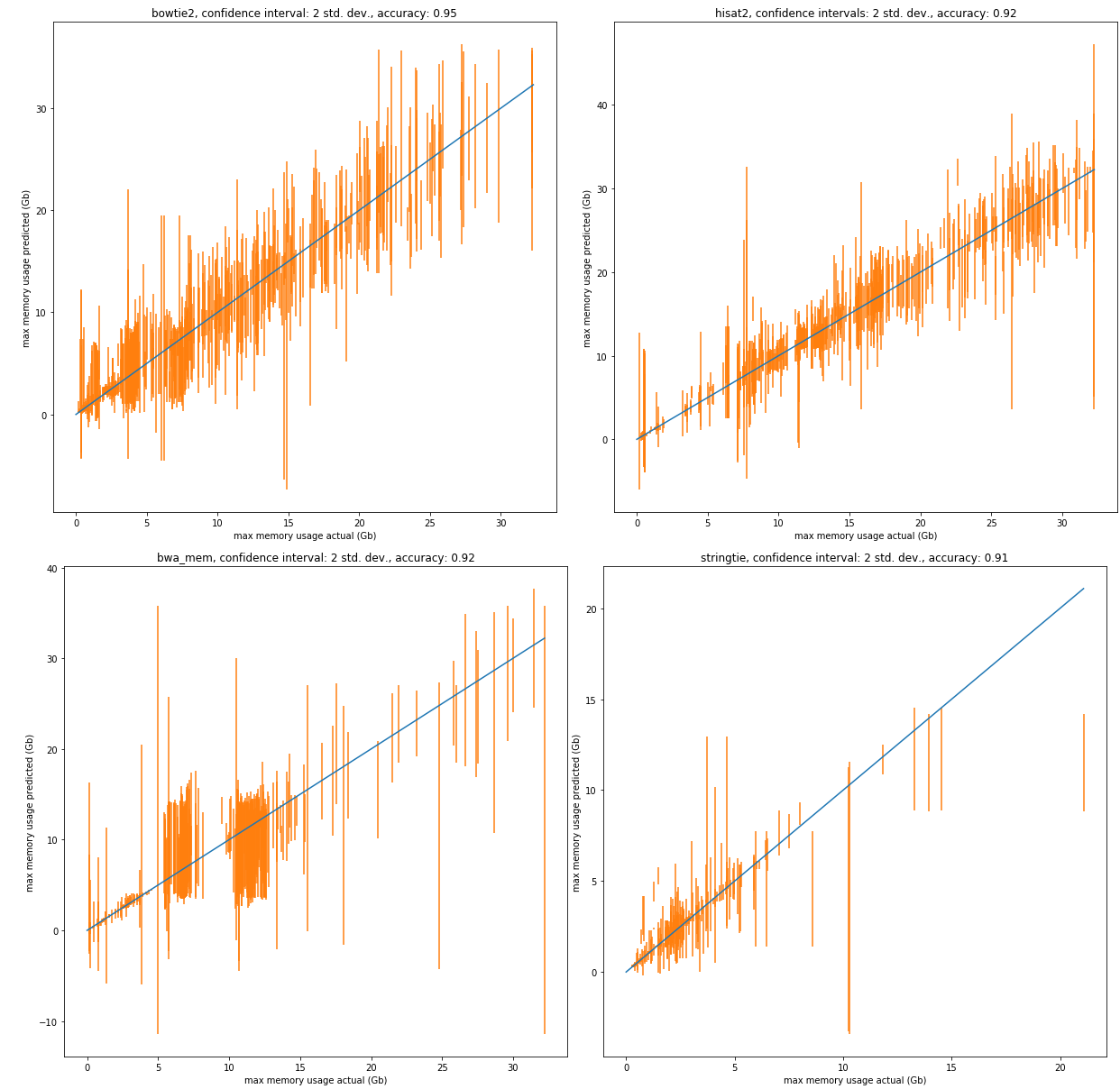
Galaxy Main began collecting memory use data in 2018. Because of this, we do not have as large of a dataset for memory usage of jobs as we do for runtimes. Consequently, we will focus on a subset of the most popular jobs for our predictive models. We use a cross validation of 5 on the data with the following results.
| tool | number of jobs in dataset | r2 score (mean) | accuracy: 1 std. dev. | accuracy: 2 std. dev. | accuracy: 3 std. dev. |
|---|---|---|---|---|---|
| bowtie2 | 3985 | 0.95 | 0.77 | 0.95 | 0.99 |
| hisat2 | 2811 | 0.96 | 0.70 | 0.92 | 0.96 |
| bwa mem | 2199 | 0.78 | 0.71 | 0.93 | 0.97 |
| stringtie | 1399 | 0.90 | 0.68 | 0.89 | 0.94 |
Below are sample predictions. The datasets are randomly split into a training set and a testing set with the testing set size of 0.2. A confidence interval of two standard deviations has been chosen for the graphs to provide a reasonable accuracy.
It is beneficial for Galaxy server administrators to know the resource requirements of a job before it is run. Allocating the correct computational resources, without using more than necessary, would lead to shorter queue times and more efficient use of resources. Moreover, for tools with high resource demand, such as those that require hundreds of gigabytes of memory, an estimation of resource requirement could detect whether a certain job will run to completion or fail.
The runtime of a job is hardware specific. It mostly depends on the CPU clock, CPU cache, memory speed, and disk read/write speed. For instance, for a job with a very large output file, the disk read/write speed may be the bottleneck. Whereas a job with complex computations may have CPU clock as the bottleneck. Because of the high variability in server hardware configurations, it is doubtful that a runtime prediction API would be accurate or even useful across different servers. A reliable prediction model would have to be trained on jobs that were run on the machine in question. Rather than a generic API, an extension of the galaxy code to create a runtime prediction model trained on the server's database would be more appropriate.
On the other hand, max memory usage of a job is not hardware dependent. This is of benefit, since we can then train model on instances of jobs across all servers to create a more robust one. Here, a generic API could be reasonable.
In this paper, we introduced the Galaxy dataset and tested popular machine learning models. We included three popular ensemble models: the Extra Trees Regressor, the Gradient Boosting Regressor, and the Random Forest Regressor. We found that Random Forests perform best in the runtime prediction task.
We also presented two methods of choosing walltimes for previously unseen jobs. Quantile regression forests are more accurate in their predictions, and grant the ability to improve performance by changing the confidence of the interval estimates. However, the sizes of the confidence intervals it provides are unpredictable, and may be unuseful if the interval is very large. Random forest classifiers are less accurate, but they allow for more control over the size of the prediction intervals.
We showed that estimating the memory requirements of a job is possible using the same methods. Memory requirements are invariant to hardware specifications, and the models may more readily be applied to other Galaxy servers.
Recently, we have begun aggregating job run data on the Galaxy Telescope from external Galaxy servers. Once this data is published we plan to test the model performance on these other servers.
We also want to find the effect of processor count on runtime. Currently, every job is allotted 32 processor cores, so we do not have the data to investigate the relationship between number of processors and runtime. In the future, we plan to add random variability to the number of processor cores allotted, so that we can see how great of an effect parallelism has on these bioinformatic algorithms.
Enis Afgan, Dannon Baker, Marius van den Beek, Daniel Blankenberg, Dave Bouvier, Martin Čech, John Chilton, Dave Clements, Nate Coraor, Carl Eberhard, Björn Grüning, Aysam Guerler, Jennifer Hillman-Jackson, Greg Von Kuster, E. Rasche, Nicola Soranzo, Nitesh Turaga, James Taylor, Anton Nekrutenko, and Jeremy Goecks. The Galaxy platform for accessible, reproducible and collaborative biomedical analyses: 2016 update. Nucleic Acids Research (2016) 44(W1): W3-W10 doi:10.1093/nar/gkw343
Scikit-learn: Machine Learning in Python, Pedregosa et al., JMLR 12, pp. 2825-2830, 2011.
Hutter, Frank, et al. "Algorithm runtime prediction: Methods & evaluation." Artificial Intelligence 206 (2014): 79-111.
Matsunaga, Andréa, and José AB Fortes. "On the use of machine learning to predict the time and resources consumed by applications." Proceedings of the 2010 10th IEEE/ACM International Conference on Cluster, Cloud and Grid Computing. IEEE Computer Society, 2010.
Gupta, Chetan, Abhay Mehta, and Umeshwar Dayal. "PQR: Predicting query execution times for autonomous workload management." Autonomic Computing, 2008. ICAC'08. International Conference on. IEEE, 2008.
Breiman, Leo. "Random forests." Machine learning 45.1 (2001): 5-32.
