incucyter is an R package to read, annotate, normalise and plot IncuCyte ZOOM® metrics.
if(!library(devtools, logical.return = T)) install.packages("devtools")
if(!library(tidyverse, logical.return = T)) install.packages("tidyverse")
devtools::install_github("uhlitz/incucyter")
You can use incucyter to...
- read + annotate
- normalise
- plot
...IncuCyte ZOOM® metrics.
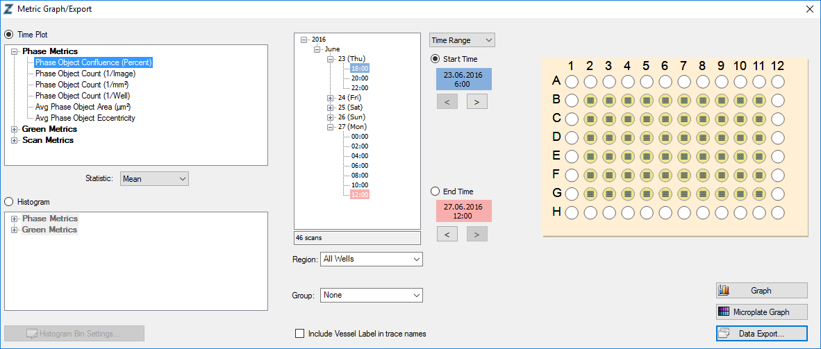
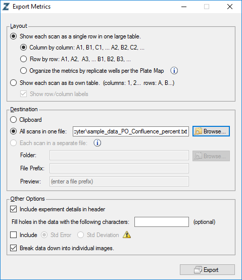
To do so, export your incucyte metrics with IncuCyte ZOOM® software using the following settings. File names are not relevant, all other settings are mandatory for incucyter to properly import the data:
Example code to read and annotate incucyte metrics:
library(tidyverse)
library(incucyter)

example_data <- system.file("extdata",
                            c("sample_data_GO_Confluence_percent.txt",
                              "sample_data_PO_Confluence_percent.txt"),
                            package = "incucyter")

example_annotation <- system.file("extdata",
                                  "sample_data_annotation.tsv",
                                  package = "incucyter")

incu_tbl <- read_incu(file = example_data,
                      annotation = example_annotation)
Your annotation table must contain four columns: Analysis_Job, Well, Treatment and Reference. You can freely add other columns and use these columns to summarise your data for plotting or summary statistics.
To annotate your table, you can use read_incu with a file path to a tab delimited annotation file or with a R data.frame.
An example annotation can look like this:
| Analysis_Job | Well | Treatment | Inhibition | siRNA | siRNA_id | siRNA_conc | HiPerfect_conc | Reference |
|---|---|---|---|---|---|---|---|---|
| Experiment_1 | B2 | EtOH | NA | NA | NA | NA | NA | B3,C3,D3 |
| Experiment_1 | C2 | EtOH | NA | NA | NA | NA | NA | B3,C3,D3 |
| Experiment_1 | D2 | EGF | NA | NA | NA | NA | NA | B3,C3,D3 |
| Experiment_1 | E2 | EGF | NA | NA | NA | NA | NA | B3,C3,D3 |
| Experiment_1 | F2 | FGF | NA | NA | NA | NA | NA | B3,C3,D3 |
| Experiment_1 | G2 | FGF | NA | NA | NA | NA | NA | B3,C3,D3 |
| Experiment_1 | B3 | 4OHT | NA | NA | NA | NA | NA | B3,C3,D3 |
| Experiment_1 | C3 | 4OHT | NA | NA | NA | NA | NA | B3,C3,D3 |
| Experiment_1 | D3 | 4OHT | NA | NA | NA | NA | NA | B3,C3,D3 |
| Experiment_1 | E3 | 4OHT | U0126 | NA | NA | NA | NA | B3,C3,D3 |
| Experiment_1 | F3 | 4OHT | U0126 | NA | NA | NA | NA | B3,C3,D3 |
| Experiment_1 | G3 | 4OHT | U0126 | NA | NA | NA | NA | B3,C3,D3 |
| Experiment_1 | B4 | 4OHT | NA | Mock | * | 10 | 2 | B4,B5 |
| Experiment_1 | B5 | 4OHT | NA | Mock | * | 10 | 2 | B4,B5 |
| Experiment_1 | B6 | 4OHT | U0126 | Mock | * | 10 | 2 | B4,B5 |
| Experiment_1 | B7 | 4OHT | U0126 | Mock | * | 10 | 2 | B4,B5 |
| Experiment_1 | B8 | EtOH | NA | Mock | * | 10 | 2 | B4,B5 |
| Experiment_1 | B9 | EtOH | NA | Mock | * | 10 | 2 | B4,B5 |
| Experiment_1 | B10 | EtOH | NA | Mock | * | 10 | 2 | B4,B5 |
| Experiment_1 | B11 | EtOH | NA | Mock | * | 10 | 2 | B4,B5 |
You can normalise your data to a reference metric and/or to a set of referece wells. For the first, calc_incu_ratios calculates all ratios between the different metrics in your table. These ratios can be plotted with plot_metric like any other metric. For the latter, norm_incu normalises your metrics to a given reference time point and a given set of reference wells (specified as a column in your annotation table, see above).
incu_tbl_comp <- calc_incu_ratios(incu_tbl)
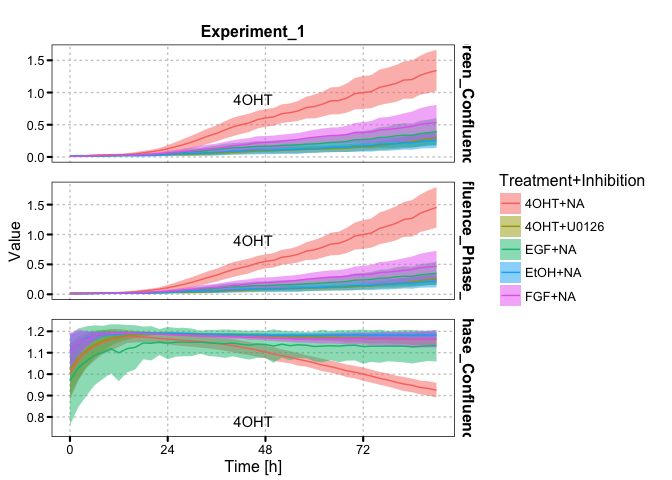
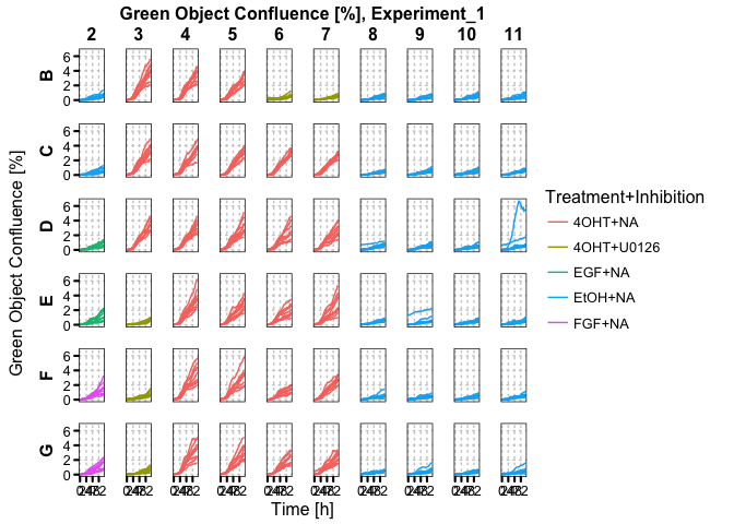
incu_tbl_comp_norm <- norm_incu(incu_tbl_comp, ref_time = 72)You can plot multiple metrics with plot_metrics or a microplate overview plot with plot_microplate.
incu_tbl_comp_norm %>%
  filter(is.na(siRNA)) %>%
  plot_metrics(color = c("Treatment", "Inhibition"),
               label = c("Treatment", "Inhibition"), summarise = T)
incu_tbl %>%
filter(Metric == "Green_Confluence") %>%
plot_microplate(color = c("Treatment", "Inhibition"))


