This is Project 5 of the Udacity Self-Driving Car Engineer Nanodegree. Vehicles on video are detected and tracked using computer vision (OpenCV) and Machine Learning techniques such as Support Vector Machines.
Main script: vehicle_detection_pipeline.py
Output video: output_videos/project_video.mp4 [Link]
- opencv
- moviepy
- matplotlib
- scikit-image
- scikit-learn
Vehicle detection and tracking is achieved by completing the following stages.
- Perform a Histogram of Oriented Gradients (HOG) feature extraction (+ color histogram and raw pixel features) on images from a labeled training set.
- Train a Linear SVM classifier using extracted features.
- Slide windows across each image, extract features, and predict vehicle presence using the trained classifier.
- Add vehicle predictions to heatmap and use thresholding values to determine whether prediction is likely to be correct.
- Classify predicted zones into a single or multiple detected vehicles and draw bounding boxes around each vehicle in the image (video frame).
file: vehicle_detection_pipeline.py
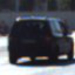
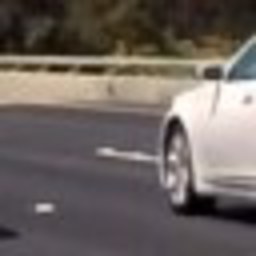
The dataset consists of labeled images (64 * 64 px) in two classes: vehicle and non-vehicle. Examples from both classes below.
| Vehicle | Vehicle | Vehicle |
|---|---|---|
 |
 |
 |
| Non-vehicle | Non-vehicle | Non-vehicle |
|---|---|---|
 |
 |
 |
Some of the images labeled non-vehicle do in fact contain vehicles. In order to qualify as a vehicle image the entire vehicle must be visible within the bounds of the image and, in addition, make a close fit to the image borders. Alternatively, this could also be an example of a dataset error.
Download the labeled dataset for vehicle and non-vehicle respectively. The data is composed from a combination of the GTI vehicle image database, the KITTI vision benchmark suite, and examples extracted from the project video itself.
HOG features are extracted using hog() from scikit-image.
from skimage.feature import hog

def hog(image, orientations=9, pixels_per_cell=(8, 8), cells_per_block=(3, 3),
        visualise=False, transform_sqrt=False, feature_vector=True, normalise=None):
A number of experiments were run to select HOG color space, image channels, and optimization parameters. The best performance in these benchmark tests was achieved using all three channels in the HSV color space in combination with the following feature extraction parameters.
orientations=12, pixels_per_cell=(8, 8), cells_per_block=(2, 2)
For the sake a brevity in this document, the full parameter optimization methodology can be found in Appendix.
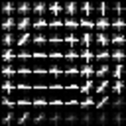
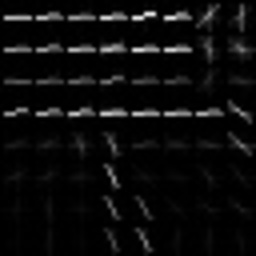
Examples of visualized HOG features for vehicle and non-vehicle classes are presented below. Only the HSV V-channel is used for visualization whereas all three HSV channels are included in the training and prediction.
| HSV V-Channel | HSV V-CH HOG | HSV V-Channel | HSV V-CH HOG |
|---|---|---|---|
 |
 |
 |
 |
HOG features are extracted along with spatial features and color histogram features. The features are normalized together using StandardScaler. The data is subsequently split into training set and test set.
from sklearn.preprocessing import StandardScaler
from sklearn.model_selection import train_test_split

X = np.vstack((car_features, non_car_features)).astype(np.float64)
y = np.hstack((np.ones(len(car_features)), np.zeros(len(non_car_features))))
self.X_scaler = StandardScaler().fit(X)
scaled_X = self.X_scaler.transform(X)

X_train, X_test, y_train, y_test = train_test_split(
scaled_X, y, test_size=0.2)The normalized data is used to train and test the classifier, in this case a Linear Support Vector Classifier.
from sklearn.svm import LinearSVC

def train(self, X_train, X_test, y_train, y_test):
    self.clf = LinearSVC()
    self.clf.fit(X_train, y_train)
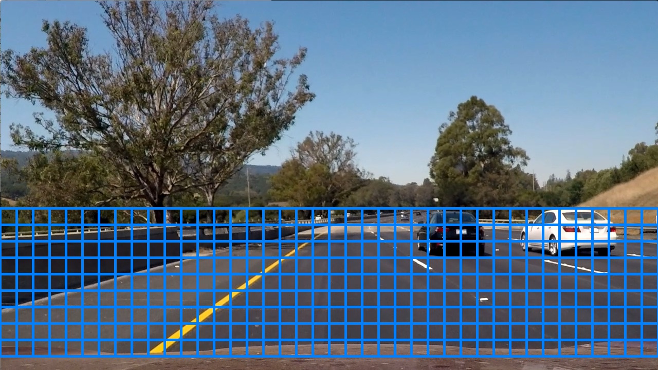
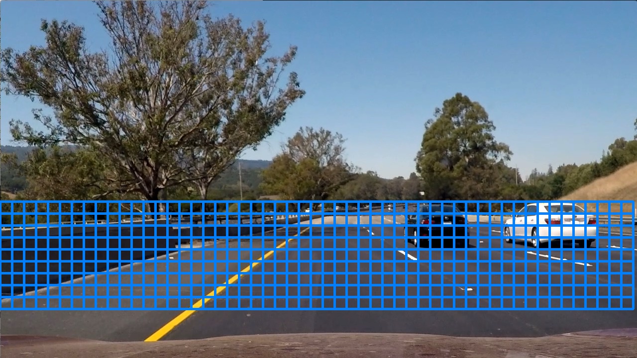
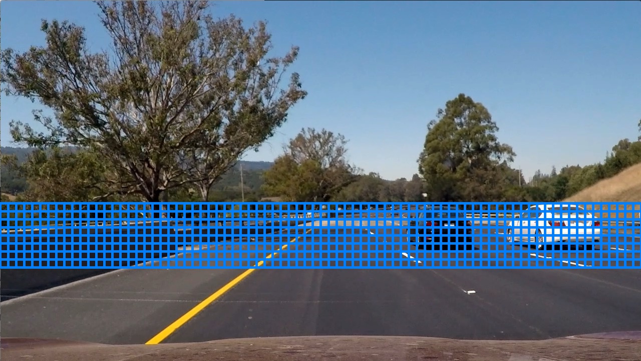
accuracy_test = self.clf.score(X_test, y_test)In order to detect vehicles in video, we scan each image (video frame) with vehicle-sized rectangular windows. The size and position of the window must be sufficiently similar to the vehicle in order to generate a match. Three sizes (128, 96, and 64 pixels) are used and snapshots are taken at regular intervals such that the windows overlap. Smaller windows scan near the center of the image (close to the horizon), and larger windows near the base of the image (close to the camera). We take care to avoid sliding windows in areas where we do not expect to find vehicles in order to save computing resources and reduce number of false positives.
| 128x128 | 96x96 | 64x64 |
|---|---|---|
 |
 |
 |
The window slider code takes as input the scan area coordinates x_start_stop, y_start_stop, window size xy_window and window overlap fraction xy_overlap. The number of windows and their corresponding coordinates are calculated.
The calculated windows are defined by the two points top_left and bottom_right i.e. ((x_min, y_min), (x_max, y_max)).
def __slide_window(x_start_stop=[None, None], y_start_stop=[None, None],
                        xy_window=(64, 64), xy_overlap=(0.5, 0.5)):

    x_width = x_start_stop[1] - x_start_stop[0]
    y_height = y_start_stop[1] - y_start_stop[0]
    x_step_size = int(xy_window[0] * (1 - xy_overlap[0]))
    y_step_size = int(xy_window[1] * (1 - xy_overlap[1]))
    x_nb_windows = int((x_width - xy_window[0]) / x_step_size + 1)
    y_nb_windows = int((y_height - xy_window[1]) / y_step_size + 1)

    windows = []
    for x_i in range(x_nb_windows):
        for y_j in range(y_nb_windows):
            top_left = (x_start_stop[0] + x_i * x_step_size, y_start_stop[0] + y_j * y_step_size)
            bottom_right = (top_left[0] + xy_window[0], top_left[1] + xy_window[1])
windows.append((top_left, bottom_right)) The content of each window is resized (64, 64) to match the classifier. Features are extracted and values normalized before prediction is performed. If prediction is positive, he window is considered hot and can be added to the heatmap.
hot_windows = []
for window in windows:
    x_min, y_min, x_max, y_max = np.ravel(window)
    resized = cv2.resize(image[y_min:y_max, x_min:x_max], (64, 64))
    features = self.feature_extractor.extract_features_from_image(resized)
    scaled_features = self.preprocessor.scale_features(features)
    if self.classifier.predict(scaled_features):
        hot_windows.append(window)
    self.heat_mapper.add_hot_windows(hot_windows)
file: vehicle_detection_pipeline.py
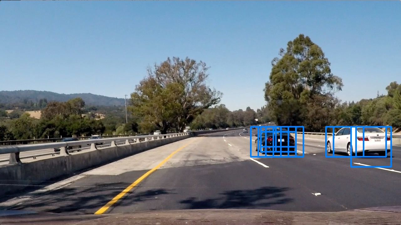
The hot_windows that are predicted as vehicles are added to a heatmap where the intensity of pixels at identical locations see their value increased (heat added). The heatmap can be filtered so that all values below a certain threshold are set to zero.
def add_hot_windows(self, hot_windows):
    heatmap = np.zeros(self.image_shape)
    for window in hot_windows:
        x_min, y_min, x_max, y_max = np.ravel(window)
        heatmap[y_min:y_max, x_min:x_max] += 1

def apply_threshold(heatmap, threshold):
    heatmap[heatmap <= threshold] = 0
return heatmap| Hot windows | Heatmap | Thresholded detection |
|---|---|---|
 |
 |
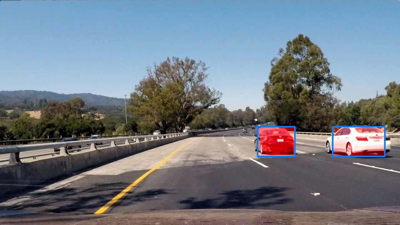 |
Pixels in the thresholded heatmap pertaining to vehicles are labelled and grouped into separate units using label(). For each of the areas the top-left pixel and the bottom-right pixel together define the detection box. An optional filter is added that can be used if false positives are more likely to produce narrow detection boxes.
from scipy.ndimage.measurements import label

def get_detection_boxes(heatmap, filter_size=(0, 0)):
    detection_boxes = []
    labels = label(heatmap)

    for car_number in range(1, labels[1] + 1):
        nonzero = (labels[0] == car_number).nonzero()
        nonzeroy = np.array(nonzero[0])
        nonzerox = np.array(nonzero[1])
        x_min, y_min, x_max, y_max = np.min(nonzerox), np.min(nonzeroy), np.max(nonzerox), np.max(nonzeroy)

        if x_max - x_min > filter_size[0] and y_max - y_min > filter_size[1]:
            detection_box = ((x_min, y_min), (x_max, y_max))
            detection_boxes.append(detection_box)
return detection_boxesWhen processing video we have the opportunity to use data from previous frames in addition to the current frame. One important benefit is that false positives classification errors and are unlikely to remain with high confidence in multiple sequential frames, thus possible to remove using a low-pass filter. Frame-to-frame optimization is achieved by Heatmap averaging and Detection box window focus.
Heatmap averaging is achieved by adding the current frame heatmap to a stack of previous heatmaps. The stack depth (and thus detection inertia/stability) is configurable by parameter nb_frames. A longer history reduces risk of losing track of a detected vehicle but also slows down initial detection.
self.heatmap_stack = np.insert(self.heatmap_stack, 0, heatmap, axis=0)
if self.heatmap_stack.shape[0] > self.nb_frames:
    self.heatmap_stack = np.delete(self.heatmap_stack, -1, axis=0)
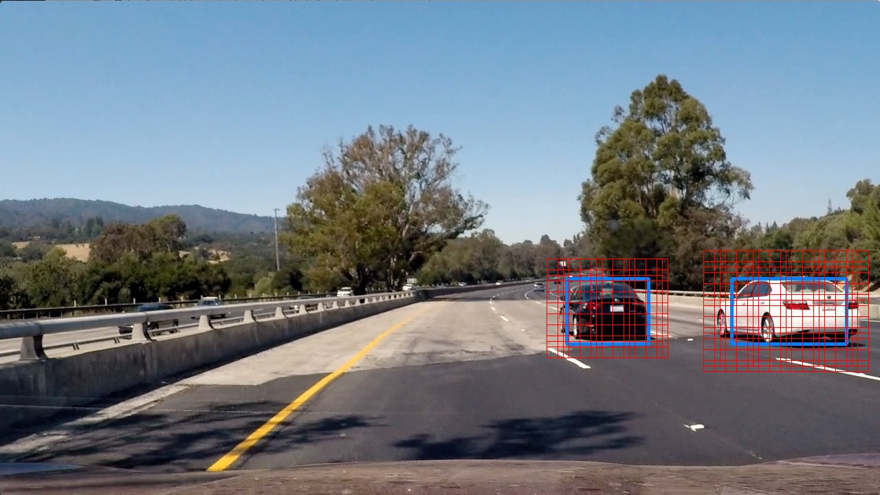
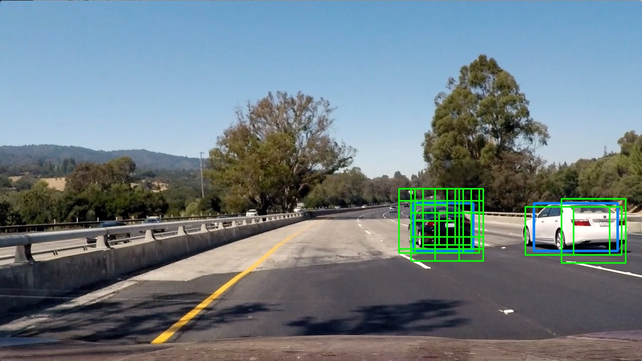
heatmap_mean = np.mean(self.heatmap_stack, axis=0)In order to avoid losing track of a detected vehicle we increase search intensity in the area around the detection box defined in the previous frame. The higher density of search windows close to the previous detection will increase the number of true positive vehicle predictions in the subsequent frame. The increased rate of correct vehicle detection can also allow for increase in heatmap thresholding, thereby reducing number of false positives.
In the left-most image (frame fn ) we see the blue detection box from frame fn-1 and the resulting extended search windows marked in red. The center image shows the hot windows resulting from the extended focus search and the right-most image presents the hot windows from the standard search in frame fn without knowledge from the previous frame. The hot windows from standard and extended window sliding are added together and passed to the heatmap.
| Extended search around detection box | Hot windows extended | Hot windows standard |
|---|---|---|
 |
 |
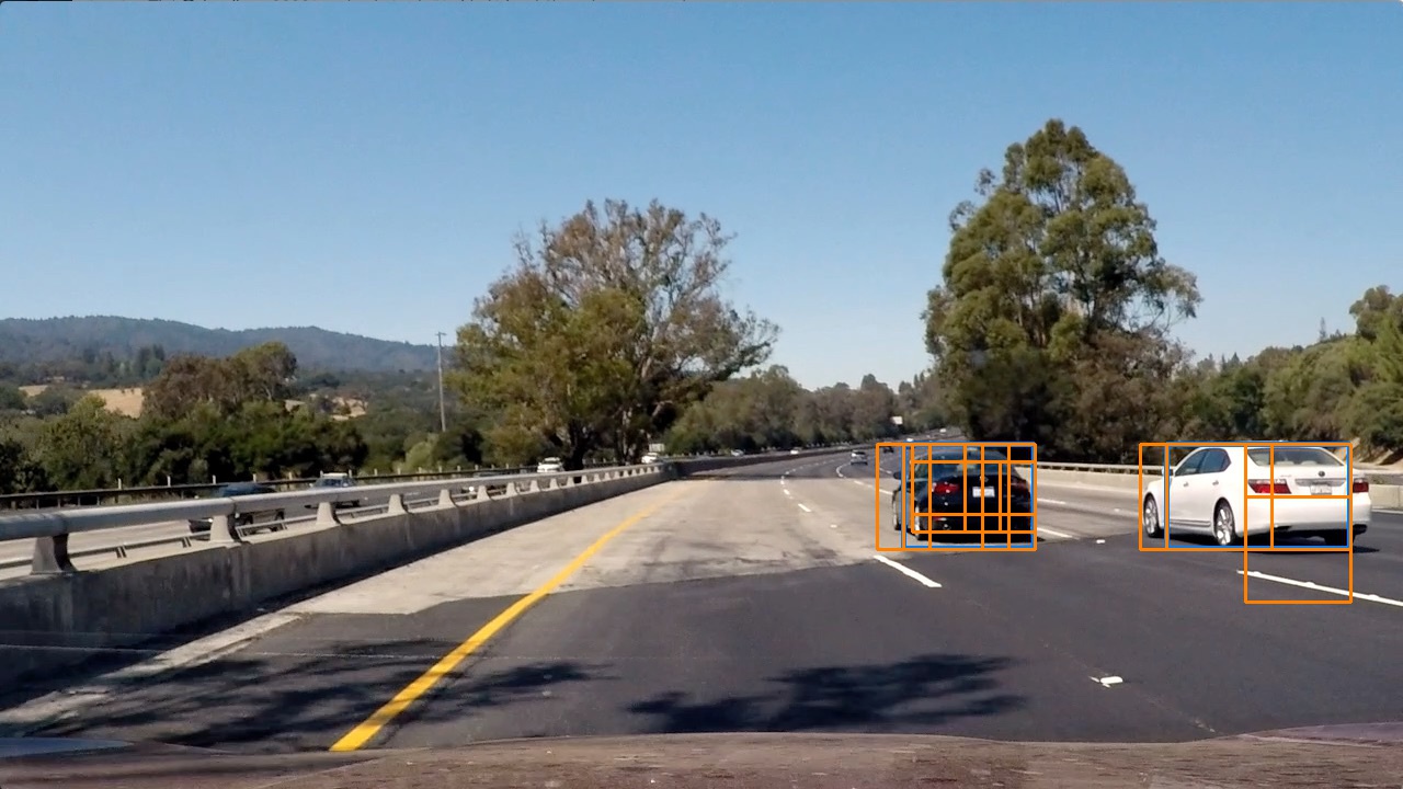 |
The difference in results comparing extended search (based on the detection from the previous frame) to standard search (from scratch) provides redundancy and stability to the detection algorithm.
def slide_window(self, img, detection_boxes=[]):
    for box in detection_boxes:
        xmin, ymin, xmax, ymax = np.ravel(box)
        dominant_dim = max(xmax-xmin, ymax-ymin)
        for dim in dimensions:
            offset = int(dominant_dim*offset_fraction)
            focus_windows = self.__slide_window(img, xy_window=(dim, dim), xy_overlap=(overlap, overlap),
                                          x_start_stop=[xmin-offset, xmax+offset],
                                          y_start_stop=[ymin-offset, ymax+offset])
windows.extend(focus_windows)The first problem to address is speed. First, the code runs on a single CPU-core. Second, the HOG feature extraction at each window is very slow. Results are measured on a Macbook Pro 15" Mid 2015 in its basic configuration of i7 quad-core Haswell CPU (full technical specs). Features are extracted for each sliding window individually. For each window we have the following breakdown.
| Spatial | Color histogram | HOG | Total | |
|---|---|---|---|---|
| Feature count | 12288 | 96 | 7056 | 19440 |
| Extraction time (ms) | 0.006 | 0.4 | 3 | 3.41 |
In a basic frame we have 644 windows, resulting in total pipeline time 2.43 s, of which 2.23 s is feature extraction. Performing the feature extraction once per frame, and only afterwards slide windows over the features would increase speed greatly.
It would be interesting to try using a CNN-classifier instead of a SVM to see if performance improves further, both accuracy and speed. Given that we are working with image classification it would certainly be worth a try.
The test accuracy of the SVM classifier was >99% which is, while not out-of-this-world, more than enough for this application if coupled with some filtering downstream. It's likely that considerable speed gains can be achieved by reducing HOG features, while still maintaining good detection performance.
When using heatmap averaging in order to reduce the number of false positives care must be taken to not include too many frames. Detection speed will otherwise suffer, and it will be much harder to detect vehicles with high speed relative to the camera. One option will be to use weighted averaging where the most recent frames carry more importance.
There was data from the project video present in the training data. It's therefore possible that performance on a previously unseen road will be worse than the level achieved in this project.