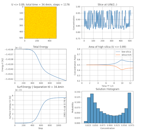
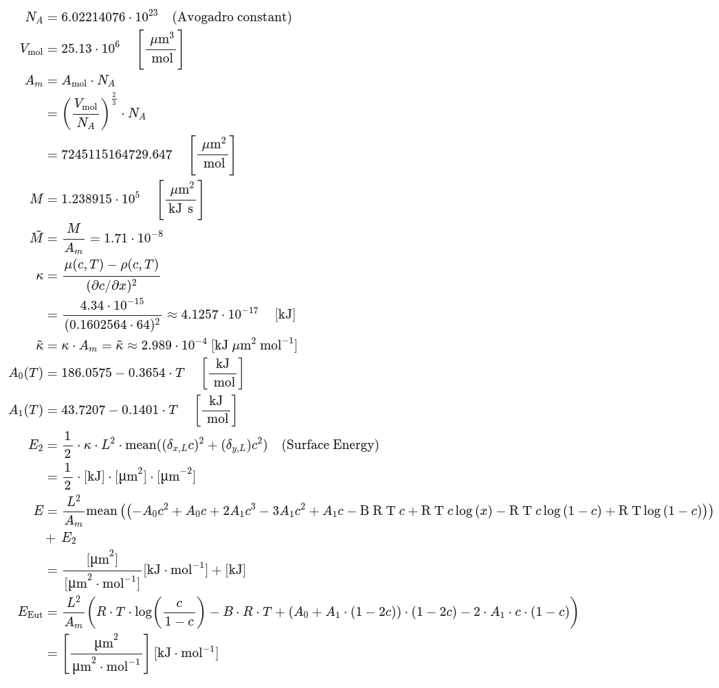
chsimpy is a python3 simulation code to solve the Cahn–Hilliard equation for phase separation of Na2O-SiO2 glasses under uncertainty. It provides an optional non-interactive graphical interface (GUI) with an optional live view of the simulation progress. Parameters can be changed via command-line interface (CLI), input data or within a jupyter notebook. Data can also be exported for post-processing and reproducibility. Results and instructions for reproduction are provided in our chsimpy-artifact github repository.
chsimpy is part of the publication: Simulation of phase separation in Na2O-SiO2 glasses under uncertainty, Henning Höllwarth, Stephan A.H. Sander, Matthias Werner, Sindy Fuhrmann, Björn Sprungk; Journal of Non-Crystalline Solids, Volume 621, 2023, ISSN 0022-3093, https://doi.org/10.1016/j.jnoncrysol.2023.122534.
For installation please read our installation instructions.
If chsimpy is installed as package, just run:
chsimpy --help
Alternatively, without package installation:
# git clone https://github.com/uncertaintyhub/chsimpy.git
# cd chsimpy
python -m chsimpy --help
The help provides information on the command-line interface (CLI) arguments:
chsimpy 1.4.1 ('--help' for command parameters)
usage: chsimpy [-h] [--version] [-N N] [-n NTMAX] [-t TIME_MAX] [-z] [-a] [--cinit CINIT] [--threshold THRESHOLD] [--temperature TEMPERATURE] [--A0 A0] [--A1 A1] [--dt DT]
               [-g {uniform,simplex,sobol,lcg}] [-s SEED] [-j JITTER] [-p PARAMETER_FILE] [--Uinit-file UINIT_FILE] [-f FILE_ID] [--no-gui] [--png] [--png-anim] [--yaml]
               [--export-csv EXPORT_CSV] [-C] [--update-every UPDATE_EVERY] [--no-diagrams]

Simulation of Phase Separation in Na2O-SiO2 Glasses under Uncertainty (solving the Cahn–Hilliard (CH) equation)

options:
  -h, --help            show this help message and exit
  --version             show program's version number and exit

Simulation:
  -N N                  Number of pixels in one domain (NxN) (default: 512)
  -n NTMAX, --ntmax NTMAX
                        Maximum number of simulation steps (might stop early, see --full-sim) (default: 1000000)
  -t TIME_MAX, --time-max TIME_MAX
                        Maximal time in minutes to simulate (ignores ntmax) (default: None)
  -z, --full-sim        Do not stop simulation early when energy falls (default: False)
  -a, --adaptive-time   Use adaptive-time stepping (approximation, experimental) (default: False)
  --cinit CINIT         Initial mean mole fraction of silica (default: 0.875)
  --threshold THRESHOLD
                        Threshold mole fraction value to determine c_A and c_B (should match --cinit) (default: 0.875)
  --temperature TEMPERATURE
                        Temperature in Kelvin (default: 923.15)
  --A0 A0               A0 value (ignores temperature) [kJ / mol] (default: None)
  --A1 A1               A1 value (ignores temperature) [kJ / mol] (default: None)
  --dt DT               Time delta of simulation (default: 3e-08)
  -g {uniform,simplex,sobol,lcg}, --generator {uniform,simplex,sobol,lcg}
                        Generator for initial random deviations in concentration (default: uniform)
  -s SEED, --seed SEED  Start seed for random number generators (default: 2023)
  -j JITTER, --jitter JITTER
                        Adds noise based on -g in every step by provided factor [0, 0.1) (much slower) (default: None)

Input:
  -p PARAMETER_FILE, --parameter-file PARAMETER_FILE
                        Input yaml file with parameter values (overwrites CLI parameters) (default: None)
  --Uinit-file UINIT_FILE
                        Initial U matrix file (csv or numpy bz2 format). (default: None)

Output:
  -f FILE_ID, --file-id FILE_ID
                        Filenames have an id like "<ID>...yaml" ("auto" creates a timestamp). Existing files will be OVERWRITTEN! (default: auto)
  --no-gui              Do not show plot window (if --png or --png-anim. (default: False)
  --png                 Export solution plot to PNG image file (see --file-id). (default: False)
  --png-anim            Export live plotting to series of PNGs (--update-every required) (see --file-id). (default: False)
  --yaml                Export parameters to yaml file (see --file-id). (default: False)
  --export-csv EXPORT_CSV
                        Solution matrix names to be exported to csv (e.g. ...="U,E2") (default: None)
  -C, --compress-csv    Compress csv files with bz2 (default: False)
  --update-every UPDATE_EVERY
                        Every n simulation steps data is plotted or rendered (>=2) (slowdown). (default: None)
  --no-diagrams         No diagrams or axes, it only renders the image map of U. (default: False)
The example file examples/example-parameters.yaml demonstrates the use of a YAML configuration for simulation parameters.
A0 and A1 are lambda functions and cannot be defined here, so you use chsimpy --A0=... --A1=... instead.
Install jupyter on your system. Perhaps further packages are required:
pip install PyQt5 ipymplWhen installing chsimpy, additional requirements also can be selected via:
pip install "chsimpy[interactive, qt5] @ git+https://github.com/uncertaintyhub/chsimpy.git"
Run in chsimpy folder:
# in /chsimpy
jupyter notebook
# notebook files can be found in examples/A python script for running parameter experiments can be found in chsimpy/experiments.py. It also can be run with chsimpy-experiment after installation of chsimpy.
It uses multi-processing to execute multiple simulation at once with varying parameters (A0, A1 in our case).
The random numbers are controlled by the seed which is defined by the iteration number, so the outcome does not depend on the parallelization.
The CLI is extended by additional arguments.
# if chsimpy is installed
chsimpy-experiment --help
# OR: within repository
python -m chsimpy.experiment -h
The help text includes the main help from above and additionally:
# (main help from above)
# ...
Experiment:
  -R RUNS, --runs RUNS  Number of Monte-Carlo runs (default: 3)
  -P PROCESSES, --processes PROCESSES
                        Runs are distributed to P processes to run in parallel (-1 = auto) (default: -1)
  --independent         Independent A0, A1 runs, i.e. A0 and A1 do not vary at the same time (default: False)
  --A-source A_SOURCE   = ['uniform', 'sobol', 'grid', '<filename>'] - Source for A0 x A1 numbers for the Monte-Carlo runs (uniform or sobol random numbers, evenly distributed grid points
[sqrt(runs) x sqrt(runs)], location of text file with row-wise A0, A1 pairs) (default: uniform)Only very basic tests can be found in tests/. It includes a small simulation, where the result is compared against the result of a pre-run non-public Matlab simulation. The validation dataset can be found in data/. There is a script tests/run-tests.sh to run the tests and things like benchmark or GUI visualization (user has to close to continue tests script).
Benchmarks of the simulation code are run by examples/benchmark.py (for more arguments check python benchmark.py --help).
python benchmark.py -N 512 -n 100 -R 3 # 512x512 domain, 100 steps, 3 runsA dockerfile is provided to create a chsimpy-based jupyter application container. Use the scripts in the docker/ folder to build and run the container.
# git clone https://github.com/uncertaintyhub/chsimpy.git
# cd chsimpy/docker
# cat build-docker.sh
export DOCKER_BUILDKIT=1 # requires docker-buildx
docker build -t chsimpy-docker:v1 .
# cat run-docker.sh
docker run -it --rm -p 8888:8888 \
     -w /home/jordan/work \
     -v $(pwd)/..:/home/jordan/work \
     chsimpy-docker:v1
Get or click on the link given in the docker run ... output above.
If the port 8888 is already in use, try -p 8889:8888 or a different port. The URL to jupyterlab must be adapted manually then:
http://127.0.0.1:8889/lab?token=xxx
The jupyterlab GUI provides a file browser of the actual chsimpy directory. The example notebook files (*.ipynb) can be found in examples/.
Of course, using the docker container is not necessary. If jupyter notebook and python packages are installed on the system (see root /requirements.txt), then just run jupyter notebook in the chsimpy directory to start the jupyter server and take the provided link.
The simulation results can be displayed as a single image of the concentration or by a set of diagrams.
chsimpy is a team project with the current maintainers and developers B. Sprungk and M. Werner. Special thanks to H. Hoellwarth, who wrote the core algorithm in Matlab and who also supported us during the migration to python. We would also like to thank S. Sander and S. Fuhrmann for her expert assistance in determining the material parameters.
The algorithm is based on the paper: Majid Ghiass, Mohammad Reza Moghbeli & Hossein Esfandian (2016) Numerical Simulation of Phase Separation Kinetic of Polymer Solutions Using the Spectral Discrete Cosine Transform Method, Journal of Macromolecular Science, Part B, 55:4, 411-425, DOI: 10.1080/00222348.2016.1153403
The project is currently under development. Feel free to open issues or pull-requests to contribute.

