To get started: Clone this repository then issue
git clone --recursive http://github.com/[username]/geometry-processing-registration.git
See introduction.
Once built, you can execute the assignment from inside the build/ using
./registration [path to mesh1.obj] [path to mesh2.obj]
In this assignment, we will be implementing a version of the iterative closest point (ICP), not to be confused with Insane Clown Posse.
Rather than registering multiple point clouds, we will register multiple triangle mesh surfaces.
This algorithm and its many variants has been used for quite some time to align discrete shapes. One of the first descriptions is given in "A Method for Registration of 3-D Shapes" by Besl & McKay 1992. However, the award-winning PhD thesis of Sofien Bouaziz ("Realtime Face Tracking and Animation" 2015, section 3.2-3.3) contains a more modern view that unifies many of the variants with respect to how they impact the same core optimization problem.
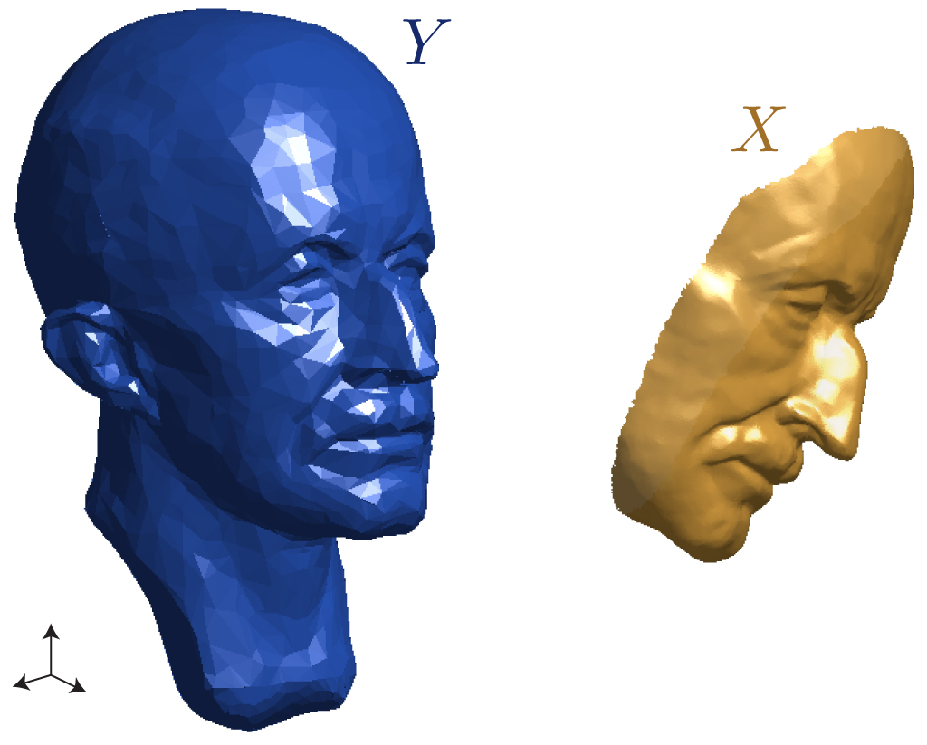
For our assignment, we will assume that we have a triangle mesh representing a
complete scan of the surface of some rigid
object and a new partial scan of
that surface
.
These meshes will not have the same number of vertices or the even the same
topology. We will first explore different ways to measure how well aligned
two surfaces are and then how to optimize the rigid alignment of the partial
surface to the complete surface
.
We would like to compute a single scalar number that measures how poorly two surfaces are matched. In other words, we would like to measure the distance between two surfaces. Let's start by reviewing more familiar distances:
The usually Euclidean distance between two points and
is the
norm of their difference :
When we consider the distance between a point and some larger object
(a line,
a circle, a surface), the natural extension is to take the distance to the
closest point
on
:
written in this way the
infimum considers all
possible points and keeps the minimum distance. We may equivalently write
this distance instead as simply the point-to-point distance between
and
the closest-point projection
:
If is a smooth surface, this projection will also be an orthogonal
projection.
We might be tempted to define the distance from surface to
as the
infimum of point-to-projection distances over all points
on
:
but this will not be useful for registering two surfaces: it will measure zero
if even just a single point of happens to lie on
. Imagine the noses of
two faces touching at their tips.
Instead, we should take the supremum of point-to-projection distances over
all points on
:
This surface-to-surface distance measure is called the directed Hausdorff
distance. We may interpret
this as taking the worst of the best: we
let each point on
declare its shortest distance to
and then keep
the longest of those.
It is easy to verify that will only equal zero if all
points on
also lie exactly on
.
The converse is not true: if there may still be
points on
that do not lie on
. In other words, in general the directed
Hausdorff distance from surface
to surface
will not equal the Hausdorff
distance from surface
to surface
:
We can approximate a lower bound on the Hausdorff distance between two meshes
by densely sampling surfaces and
. We will discuss sampling methods,
later. For now consider that we have chosen a set
of
points on
(each point might lie at a vertex, along an edge, or inside a triangle). The
directed Hausdorff distance from
to another triangle mesh
must be
greater than the directed Hausdorff distance from this point
cloud
to
:
where we should be careful to ensure that the projection of the
point
onto the triangle mesh
might lie at a vertex, along an edge or
inside a triangle.
As our sampling becomes denser and denser on
this lower bound will
approach the true directed Hausdorff distance. Unfortunately, an efficient
upper bound is significantly more difficult to design.
Even if it were cheap to compute, Hausdorff distance is difficult to
optimize when aligning two surfaces. If we treat the Hausdorff distance
between surfaces and
as an energy to be minimized, then only change to
the surfaces that will decrease the energy will be moving the (in general)
isolated point on
and isolated point on
generating the maximum-minimum
distance. In effect, the rest of the surface does not even matter or effect the
Hausdorff distance. This, or any type of
norm, will be much more
difficult to optimize.
Hausdorff distance can serve as a validation measure, while we turn to
norms for optimization.
We would like a distance measure between two surfaces that — like Hausdorff
distance — does not require a shared parameterization. Unlike Hausdorff
distance, we would like this distance to diffuse the measurement over the
entire surfaces rather than generate it from the sole worst offender. We can
accomplish this by replacing the supremum in the Hausdorff distance ()
with a integral of squared distances (
). Let us first define a directed
closest-point distance from a surface
to another surface
, as the
integral of the squared distance from every point
on
to its
closest-point projection
on the surfaces
:
This distance will only be zero if all points on also lie on
, but when
it is non-zero it is summing/averaging/diffusing the distance measures of all
of the points.
This distance is suitable to define a matching energy, but is not necessarily
welcoming for optimization: the function inside the square is non-linear. Let's
dig into it a bit. We'll define a directed matching energy
from
to
to be the squared directed
closest point distance from
to
:
where we introduce the proximity function defined simply as the
vector from a point
to its closest-point projection onto
:
Suppose was not a surface, but just a single point
. In this
case,
is clearly linear in
.
Similarly, suppose was an infinite
plane
defined by some point
on the plane and the plane's unit normal vector
. Then
is also linear in
.
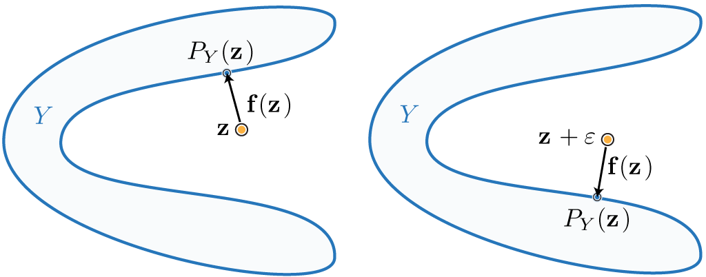
But in general, if is an interesting surface
will be non-linear; it
might not even be a continuous function.
In optimization, a common successful strategy to minimize energies composed of
squaring a non-linear functions is to
linearize the function about a
current input value (i.e., a current guess
), minimize the energy built
from this linearization, then re-linearize around that solution, and then
repeat.
This is the core idea behind gradient descent and the Gauss-Newton methods:
minimize f(z)^{2}
  z_{0} ← initial guess
  repeat until convergence
    f_{0} ← linearize f(z) around z_{0}
    z_{0} ← minimize f_{0}(z)^{2}
Since our is a geometric function, we can derive its linearizations
geometrically.
If we make the convenient—however unrealistic—assumption that in the
neighborhood of the closest-point projection of the current guess
the surface
is simply the point
(perhaps imagine that
is makes a sharp needle-like point at
or that
is very far away
from
), then we can approximate
in the proximity of our current
guess
as the vector between the input point
and
:
In effect, we are assuming that the surface is constant function of its
parameterization:
.
Minimizing iteratively using this linearization of
is equivalent to gradient
descent. We have simply derived
our gradients geometrically.
If we make make a slightly more appropriate assumption that in the neighborhood
of the the surface
is a plane, then we can improve this
approximation while keeping
linear in
:
where the plane that best approximates locally near
is the
tangent plane defined by the
normal vector
at
.
Minimizing iteratively using this linearization of
is equivalent to the
Gauss-Newton method. We
have simply derived our linear approximation geometrically.
Equipped with these linearizations, we may now describe an optimization
algorithm
for minimizing the matching energy between a surface and another surface
.
So far we have derived distances between a surface and another surface
.
In our rigid alignment and registration problem, we would like to
transform one
surface
into a new surface
so that it best aligns with/matches
the other surface
. Further we require that
is a rigid transformation:
for some rotation matrix
(i.e., an orthogonal matrix with determinant
1) and translation vector
.
Our matching problem can be written as an optimization problem to find the best
possible rotation and translation
that match surface
to surface
:
Even if is a triangle mesh, it is difficult to integrate over all
points on the surface of
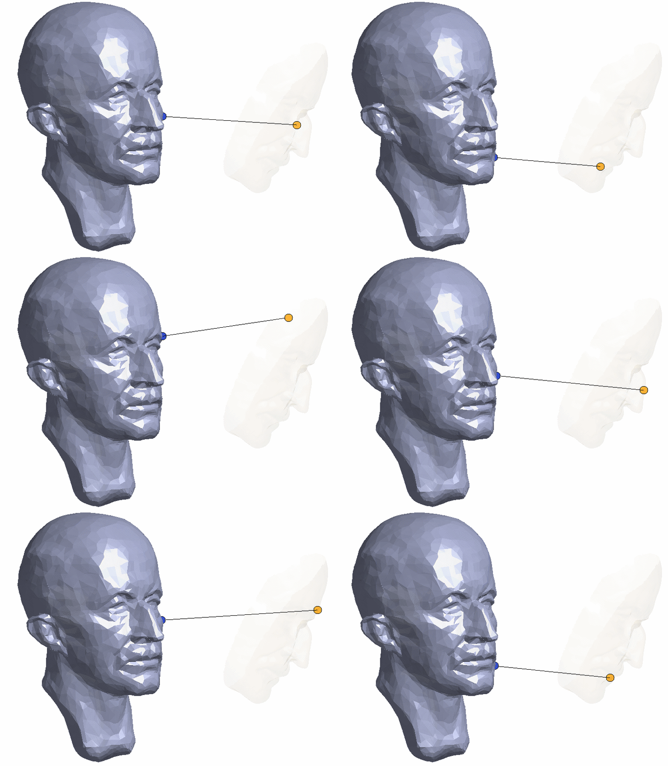
. At any point, we can approximate this energy by
summing over a point-sampling of
:
where is a set of
points on
so that each point
might lie at a vertex, along an edge, or inside a triangle. We defer discussion
of how to sample a triangle mesh surface.
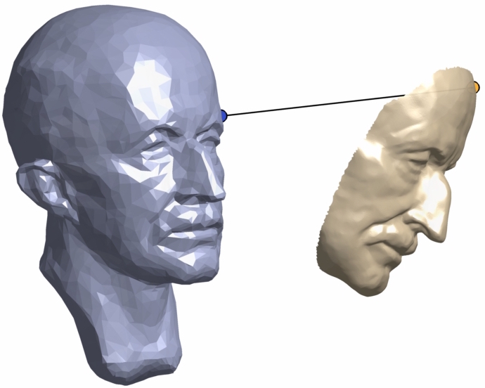
As the name implies, the method proceeds by iteratively finding the closest
point on to the current rigid transformation
of each sample
point
in
and then minimizing the linearized energy to update the
rotation
and translation
.
If V_X and F_X are the vertices and faces of a triangle mesh surface
(and correspondingly for
), then we can summarize a generic ICP algorithm in
pseudocode:
icp V_X, F_X, V_Y, F_Y
  R,t \Leftarrow  initialize (e.g., set to identity transformation)
  repeat until convergence
    X \Leftarrow  sample source mesh (V_X,F_X)
    P0 \Leftarrow  project all X onto target mesh (V_Y,F_Y)
    R,t \Leftarrow  update rigid transform to best match X and P0
    V_X \Leftarrow  rigidly transform original source mesh by R and t
We would like to find the rotation matrix and
translation vector
that best aligns a given a set of points
on the source mesh and their current closest points
on the target mesh. We have two choices for linearizing our matching energy:
point-to-point (gradient descent) and point-to-plane (Gauss-Newton).
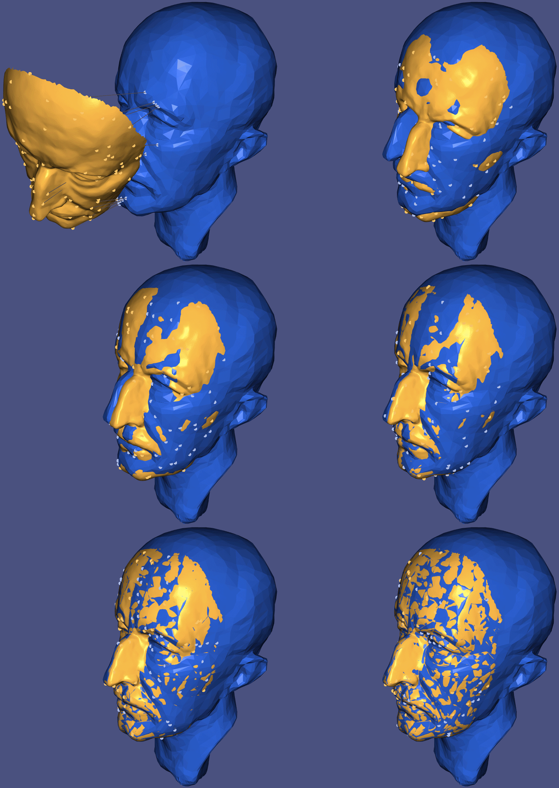
ICP using the point-to-point matching energy linearization is slow to converge.
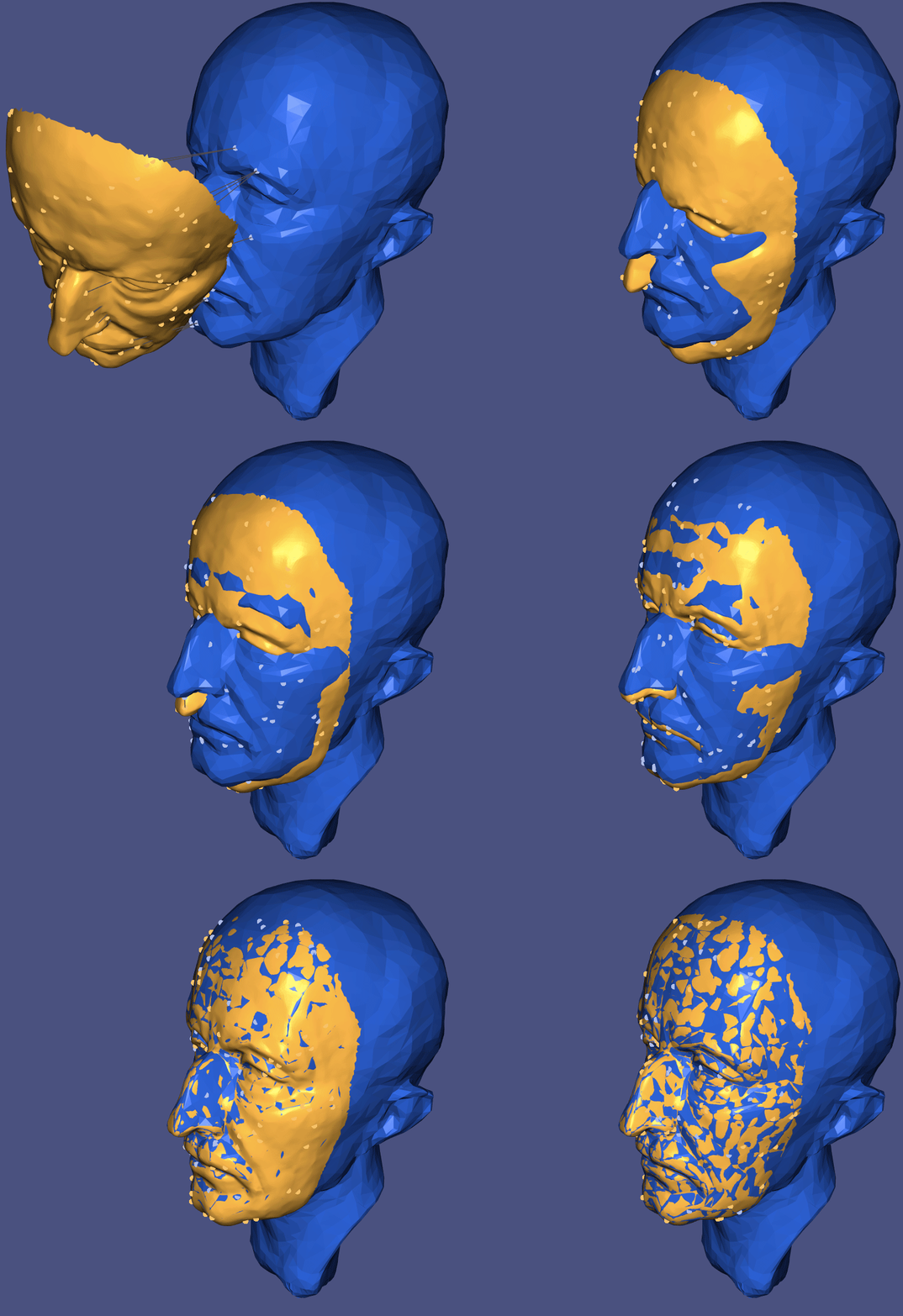
ICP using the point-to-plane matching energy linearization is faster.
In either case, this is still a non-linear optimization problem. This time due to the constraints rather than the energy term.
In an effort to provide an alternative from "Least-Squares Rigid Motion Using SVD" [Sorkine 2009], this derivation purposefully avoids the trace operator and its various nice properties.
The point-to-point (gradient descent) rigid matching problem solves:
This is a variant of what's known as a Procrustes problem, named after a mythical psychopath who would kidnap people and force them to fit in his bed by stretching them or cutting off their legs. In our case, we are forcing to be perfectly orthogonal (no "longer", no "shorter").
This energy is quadratic in and there are no other constraints on
. We can immediately solve for the optimal
— leaving
as an unknown — by
setting all derivatives with respect to unknowns in
to zero:
where is a vector ones and
computes the squared Frobenius norm of the matrix
(i.e., the sum of all squared element values. In MATLAB syntax:
sum(sum(A.^2))). Setting the partial derivative with respect to of this quadratic energy to zero finds the minimum:
Rearranging terms above reveals that the optimal is the vector aligning
the centroids of the points in
and the points in
rotated by the — yet-unknown —
. Introducing
variables for the respective centroids
and
, we can write the
formula for the optimal
:
Now we have a formula for the optimal translation vector in terms of the
unknown rotation
. Let us
substitute this formula
for all occurrences of
in our energy written in its original summation
form:
where we introduce where the ith row contains the
relative position of the ith point to the centroid
: i.e.,
(and analagously for
).
Now we have the canonical form of the orthogonal procrustes problem. To find the optimal rotation matrix , using the associativity property of the Frobenius norm, we will massage the terms in the minimization until we have a maximization problem involving the Frobenius inner-product of the unknown rotation
and covariance matrix of
and
:
where is the Frobenius inner product of
and
(i.e., the sum of all per-element products. In MATLAB syntax:
sum(sum(A.*B))). This can be further reduced:
Hint: 👁️
Letting . We can understand this problem as projecting the covariance matrix
to the nearest rotation matrix
.
Question: How can we prove that
?
Hint: Recall some linear algebra properties:
- Matrix multiplication (on the left) can be understood as acting on each column:
,
- The Kronecker product
$\mathbf{I} \otimes \mathbf{A}$ of the identity matrix$\mathbf{I}$ of size$k$ and a matrix$\mathbf{A}$ simply repeats$\mathbf{A}$ along the diagonal k times. In MATLAB,repdiag(A,k),- Properties 1. and 2. imply that the vectorization of a matrix product
can be written as the Kronecker product of the #-columns-in-
identity matrix and
times the vectorization of
:
,
- The transpose of a Kronecker product is the Kronecker product of transposes:
,
- The Frobenius inner product can be written as a dot product of vectorized matrices:
,
- Properties 3., 4., and 5. imply that Frobenius inner product of a matrix
and the matrix product of matrix
and
is equal to the Frobenius inner product of the matrix product of the transpose of
and
and the matrix
: .
Any matrix can be written in terms of its singular value decomposition. Let's do this for our covariance matrix: , where
are orthonormal matrices and
is a non-negative diagonal matrix:
We can use the permutation property of Frobenius inner product again to move the products by and
from
the right argument to the left argument:
Now, and
are both
orthonormal, so multiplying
them against a rotation matrix
does not change its orthonormality. We can
pull them out of the maximization if we account for the reflection they might
incur: introduce
with
.
This implies that the optimal rotation for the original problem is recovered
via
. When we move the
inside, we now
look for an orthonormal matrix
that is a reflection (if
) or a rotation (if
):
This ensures that as a result will be a rotation:
.
Recall that
is a non-negative diagonal matrix of singular values sorted so that the smallest value is in the bottom right corner.
Because is orthonormal, each column (or row) of
must have unit norm.
Placing a non-zero on the off-diagonal will get "killed" when multiplied by the
corresponding zero in
. So the optimal choice of
is to set all values to
zero except on the diagonal. If
, then we should set
one (and only one) of these values to
. The best choice is the bottom right
corner since that will multiply against the smallest singular value in
(add
negatively affect the maximization the least):
Finally, we have a formula for our optimal rotation:
The point-to-plane (Gauss-Newton) rigid matching problem solves:
where is the unit normal at the located closest point
. Since
is a unit vector the norm is only measuring the proceeding term
, so we can reduce this problem to:
Unlike the point-to-point problem above, there is no closed-form solution to this problem. Instead we will ensure that
that is not just any
matrix, but a rotation matrix by iterative linearization.
If we simply optimize the 9 matrix entries of directly, the result will be far from a rotation matrix: for example, if
is a twice scaled version of
, then this unconstrained optimization would happily declare the entries of
to describe a (non-orthonormal) scaling matrix.
Instead, we linearize the constraint that stays a rotation matrix and work with a reduced set of variables.
Any rotation in 3D can be written as scalar rotation angle
around a rotation axis defined by a unit vector
.
If , we know that a rotation by
can be written as:
For a general, rotation axis , we can write a generalized axis-angle to matrix formula:
where is the skew-symmetric cross product matrix of
so that
In this form, we can linearize by considering a small change in and
:
By defining , we can write this in terms of only three simple scalar variables:
or written in terms of its action on a vector , we can simply write in terms of the cross product:
If we apply our linearization of to the point-to-plane distance
linearization of the matching energy, our minimization is:
Let's gather a vector of unknowns: . Then we can use properties of the triple product to rewrite our problem as:
Expanding all terms, moving the summations inside like terms, we can expose this in familiar quadratic energy minimization form:
Gather coefficients into and
, we have a compact quadratic minimization problem in
:
whose solution is revealed as .
Question: How do we know that
is a minimizer and not a maximizer of the quadratic expression above?
Hint: 🥣
Question: For our problem can we reasonably assume that
will be invertible?
Hint: 🎰
Solving this small system gives us our translation vector
and the linearized rotation
. If we simply assign
then our transformation will not be rigid. Instead, we should recover the
axis and angle of rotation from via
and
and then update our rotation via the axis-angle to matrix formula above. Because we used a
linearization of the rotation constraint, we cannot assume that we have
successfully found the best rigid transformation. To converge on an optimal
value, we must set
and repeat
this process (usually 5 times or so is sufficient).
Our last missing piece is to sample the surface of a triangle mesh with
faces uniformly randomly. This allows us to approximate continuous integrals
over the surface
with a summation of the integrand evaluated at a finite
number of randomly selected points. This type of numerical
integration is called the
Monte Carlo method.
We would like our random
variable to have a
uniform probability density
function
, where
is the surface
area of the triangle mesh
. We
can achieve this by breaking the problem into two steps: uniformly sampling in
a single triangle and sampling triangles non-uniformly according to their
area.
Suppose we have a way to evaluate a continuous random point in a triangle
with uniform probability density function
and we have a
away to evaluate a discrete random triangle index
with discrete
probability
distribution
, then the joint probability of evaluating a certain triangle
index
and then uniformly random point in that triangle
is indeed
uniform over the surface:
In order to pick a point uniformly randomly in a triangle with corners we will first pick a point uniformly randomly in the
parallelogram formed by
reflecting
across the line
:
where are uniformly sampled from the unit interval
. If
then the point
above will lie in the reflected triangle rather than the
original one. In this case, preprocess
and
by setting
and
to reflect the point
back into the original triangle.
Assuming we know how to draw a continuous uniform random variable from
the unit interval
, we would now like to draw a discrete random
triangle index
from the sequence
with likelihood proportional to
the relative area of each triangle in the mesh.
We can achieve this by first computing the cumulative
sum of the relative
areas:
Then our random index is found by identifying the first entry in whose
value is greater than a uniform random variable
. Since
is sorted,
locating this entry can be done in
time.
Try profiling your code. Where is most of the computation time spent?
If you have done things right, the majority of time is spent computing
point-to-mesh distances. For each query point, the computational
complexity of
computing its distance to a mesh with faces is
.
This can be dramatically improved (e.g., to on average) using an
space partitioning data
structure such as a kd tree, a
bounding volume
hierarchy, or
spatial hash.
You could follow this assignment from our graphics course to learn how to implement an AABB tree.
This reading task is not directly graded, but it's expected that you read and understand sections 3.2-3.3 of Sofien Bouaziz's PhD thesis "Realtime Face Tracking and Animation" 2015. Understanding this may require digging into wikipedia, other online resources or other papers.
You may not use the following libigl functions:
igl::AABBigl::fit_rotationsigl::hausdorffigl::iterative_closest_pointigl::point_mesh_squared_distanceigl::point_simplex_squared_distanceigl::polar_decigl::polar_svd3x3igl::polar_svdigl::random_points_on_meshigl::rigid_alignmentEigen::umeyama
You are encouraged to use the following libigl functions:
igl::cumsumcomputes cumulative sumigl::doubleareacomputes triangle areasigl::per_face_normalscomputes normal vectors for each triangle face
Generate n random points uniformly sampled on a given triangle mesh with
vertex positions VX and face indices FX.
Compute the distance d between a given point x and the closest point p on
a given triangle with corners a, b, and c.
Compute the distances D between a set of given points X and their closest
points P on a given mesh with vertex positions VY and face indices FY.
For each point in P also output a corresponding normal in N.
It is OK to assume that all points in
Plie inside (rather than exactly at vertices or exactly along edges) for the purposes of normal computation inN.
Compute a lower bound on the directed Hausdorff distance from a given mesh
(VX,FX) to another mesh (VY,FY). This function should be implemented by
randomly sampling the mesh.
Given a matrix
M, find the closest rotation matrix R.
Given a set of source points X and corresponding target points P, find the optimal rigid transformation (R,t) that aligns X to P, minimizing the point-to-point matching energy.
Given a set of source points X and corresponding target points P and their
normals N, find the optimal rigid transformation (R,t) that aligns X to
planes passing through P orthogonal to N, minimizing the point-to-point
matching energy.
Conduct a single iteration of the iterative closest point method align
(VX,FX) to (VY,FY) by finding the rigid transformation (R,t)
minimizing the matching energy.
The caller can specify the number of samples num_samples used to approximate
the integral over and specify the
method (point-to-point or
point-to-plane).
