This is a Python implementation of the Price Weller Pinkel (PWP) ocean mixed layer model. This code is based on the MATLAB verision of the PWP model, originally written by Peter Lazarevich and Scott Stoermer (U. Rhode Island) and later modified by Byron Kilbourne (University of Washington) and Sarah Dewey (University of Washington).
For a detailed description of the theory behind the model, the best source is the original Price et al. (1986) paper that introduced the model. A much shorter review of the algorithm is provided in the HYCOM documentation for the PWP; a google search may yield better sources.
The code presented here is functionally similar to its MATLAB equivalent (see matlab_files/PWP_Byron.m), but I have made significant changes to the code organization and flow. One big difference is that this code is split into two files: PWP.py and PWP_helper.py.
PWP.py contains the core numerical algorithms for the PWP model and is mostly a line-by-line translation of the original MATLAB code.
PWP_helper.py contains helper functions to facilitate model initialization, output analysis and other miscellaneous tasks. Many of these functions were introduced in this implementation.
DISCLAIMER: I did this python translation as a personal exercise, so I would recommend thoroughly examining this code before adopting it for your personal use. Feel free to leave a note under the issues tab if you encounter any problems.
To run this code, you'll need Python 3 (might work with later versions of Python 2) and the following libraries:
- Numpy
- Scipy
- Matplotlib
- xarray
- seawater
The first three modules are available with popular python distributions such as Anaconda and Canopy. You can get the other two modules via pip install from the unix command line:
pip install xarray
pip install seawater
Once these libraries are installed, you should be able to run the demos that are mentioned below.
As mentioned above, the code is split across two files PWP.py and PWP_helper.py. PWP.py contains all the numerical algorithms while PWP_helper.py has a few auxillary functions. The order of operations is as follows:
- Set and derive model parameters. (See set_params function in PWP_helper.py).
- Prepare forcing and profile data for model run (see prep_data function in PWP_helper.py).
- Iterate the PWP model:
- apply heat and salt fluxes.
- apply wind stress (momentum flux).
- apply drag associated with internal-inertial wave dispersion.
- apply bulk Richardson mixing.
- apply gradient Richardson mixing.
- apply diapycnal diffusion (if ON).
- Save results to an output file.
- Make simple plots to visualize the results.
If you wish to obtain a deeper understanding of how this code works, the PWP.run() function would be a good place to start.
The PWP model requires two input netCDF files: one for the surface forcing and another for the initial CTD profile. The surface forcing file must have the following data fields:
- time: sample time (days).
- sw: net shortwave radiation (W/m2)
- lw: net longwave radiation (W/m2)
- qlat: latent heat flux (W/m2)
- qsens: sensible heat flux (W/m2)
- tx: eastward wind stress (N/m2)
- ty: northward wind stress (N/m2)
- precip: precipitation rate (m/s)
For fluxes, positive values should correspond to heat/freshwater gained by the ocean. Note that the MATLAB version of this code uses a different sign convention.
Freshwater flux due to evaporation is computed from qlat.
The time data field should contain a 1-D array representing fraction of day. For example, for 6 hourly data, this should be a number series that increases in steps of 0.25, such as np.array([1.0, 1.25, 1.75, 2.0, 2.25...]).
The initial profile file should have the following data fields:
- z: 1-D array of depth levels (m)
- t: 1-D array containing temperature profile (degrees celsius)
- s: 1-D array containing salinity profile (PSU)
- lat: Array with float representing the latitude of profile. e.g.
prof_data['lat'] = [45] #45N
Examples of both input files are provided in the input directory.
For examples of how to run the code, see the run_demo1() and run_demo2() functions in PWP_helper.py. run_demo2() is illustrated below.
The main model parameters and their defaults are listed below. See test runs below for examples of how to change these settings:
- dt: time-step increment. Input value in units of hours, but this is immediately converted to seconds. [3 hours]
- dz: depth increment (meters). [1m]
- max_depth: Max depth of vertical coordinate (meters). [100]
- mld_thresh: Density criterion for MLD (kg/m3). [1e-4]
- dt_save: time-step increment for saving to file (multiples of dt). [1]
- rb: critical bulk richardson number. [0.65]
- rg: critical gradient richardson number. [0.25]
- rkz: background vertical diffusion (m**2/s). [0.]
- beta1: longwave extinction coefficient (meters) [0.6]
- beta2: shortwave extinction coefficient (meters). [20]
- winds_ON: True/False flag to turn ON/OFF wind forcing. [True]
- emp_ON: True/False flag to turn ON/OFF freshwater forcing. [True]
- heat_ON: True/False flag to turn ON/OFF surface heat flux forcing. [True]
- drag_ON: True/False flag to turn ON/OFF current drag due to internal-inertial wave dispersion. [True]
This example uses data from SO_profile1.nc and SO_met_30day.nc, which contain the initial profile and surface forcing data respectively. For the initial profile, we use the first profile collected by Argo float 5904469. This profile was recorded in the Atlantic sector of the Southern Ocean (specifically, -53.5$^{\circ}$ N and 0.02$^{\circ}$ E) on December 11, 2014. For the surface forcing, we use 30 day time series of 6-hourly surface fluxes from NCEP reanalysis at the above location.
To run the demo that uses this data, you can do the following from a Python terminal
>>> import PWP_helper
>>> PWP_helper.run_demo2()
Doing this will execute the model and generate several plots.
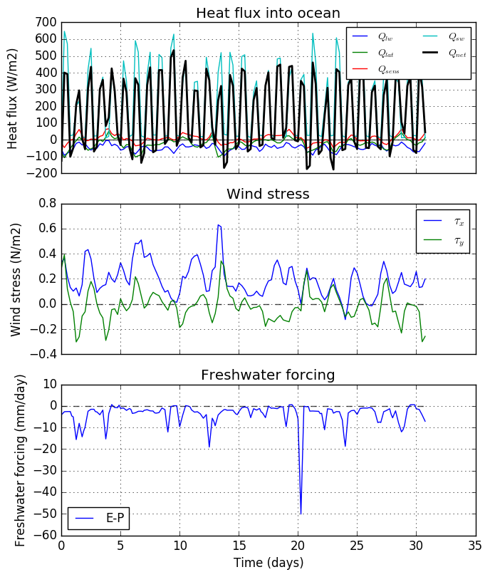
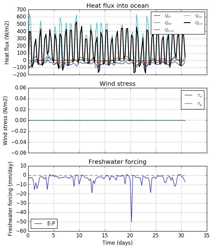
The surface forcing time series are shown below.
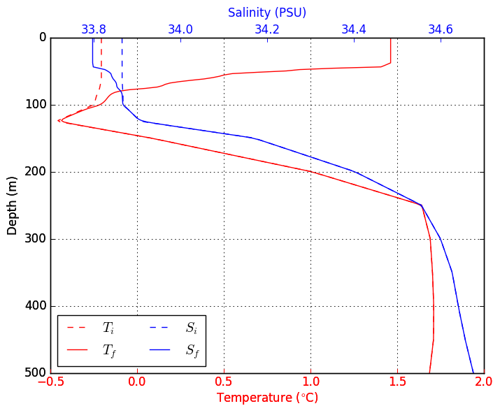
For this model run, we set the vertical diffusivity to 1x10⁻⁶ m2/s, and change the max depth and depth increment to 500m and 2m, respectively:
forcing_fname = 'SO_met_30day.nc'
prof_fname = 'SO_profile1.nc'
p={}
p['rkz']=1e-6
p['dz'] = 2.0
p['max_depth'] = 500.0
forcing, pwp_out = PWP.run(met_data=forcing_fname, prof_data=prof_fname, save_plots=True, param_kwds=p)
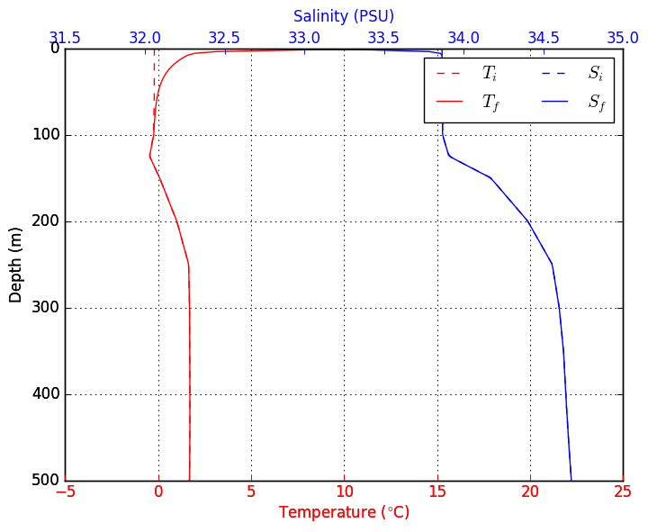
The results are displayed below.
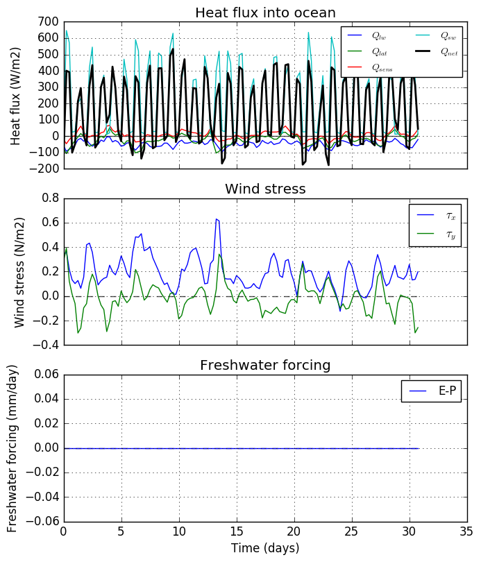
In this run, everything is the same as the previous example except that the E-P forcing is turned off. To execute this run, you can do
>>> PWP_helper.run_demo2(emp_ON=False)
The resulting surface forcing is shown below:
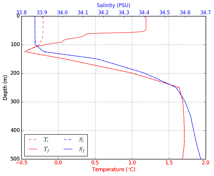
This results in the following upper ocean evolution:
As we can see, setting the freshwater flux to zero results in a final mixed layer is slightly deeper, saltier and cooler.
In this simulation, the wind forcing is turned off.
>>> PWP_helper.run_demo2(winds_ON =False)
Without wind-driven mixing, the final mixed layer depth is much shallower than the previous cases.
- Create an option to add a passive tracer to the model.
- Incorporate a rudimentary sea-ice model to provide ice induced heat and salt fluxes.
