NetCoMi (Network Comparison for Microbiome data) provides functions
for constructing, analyzing, and comparing networks suitable for the
application on microbial compositional data. The package includes
existing methods for zero handling, normalization, estimating
associations between OTU/taxa as well as dissimilarities between
samples. Furthermore, a function for constructing differential
association networks including methods for identifying differentially
associated taxa is offered.
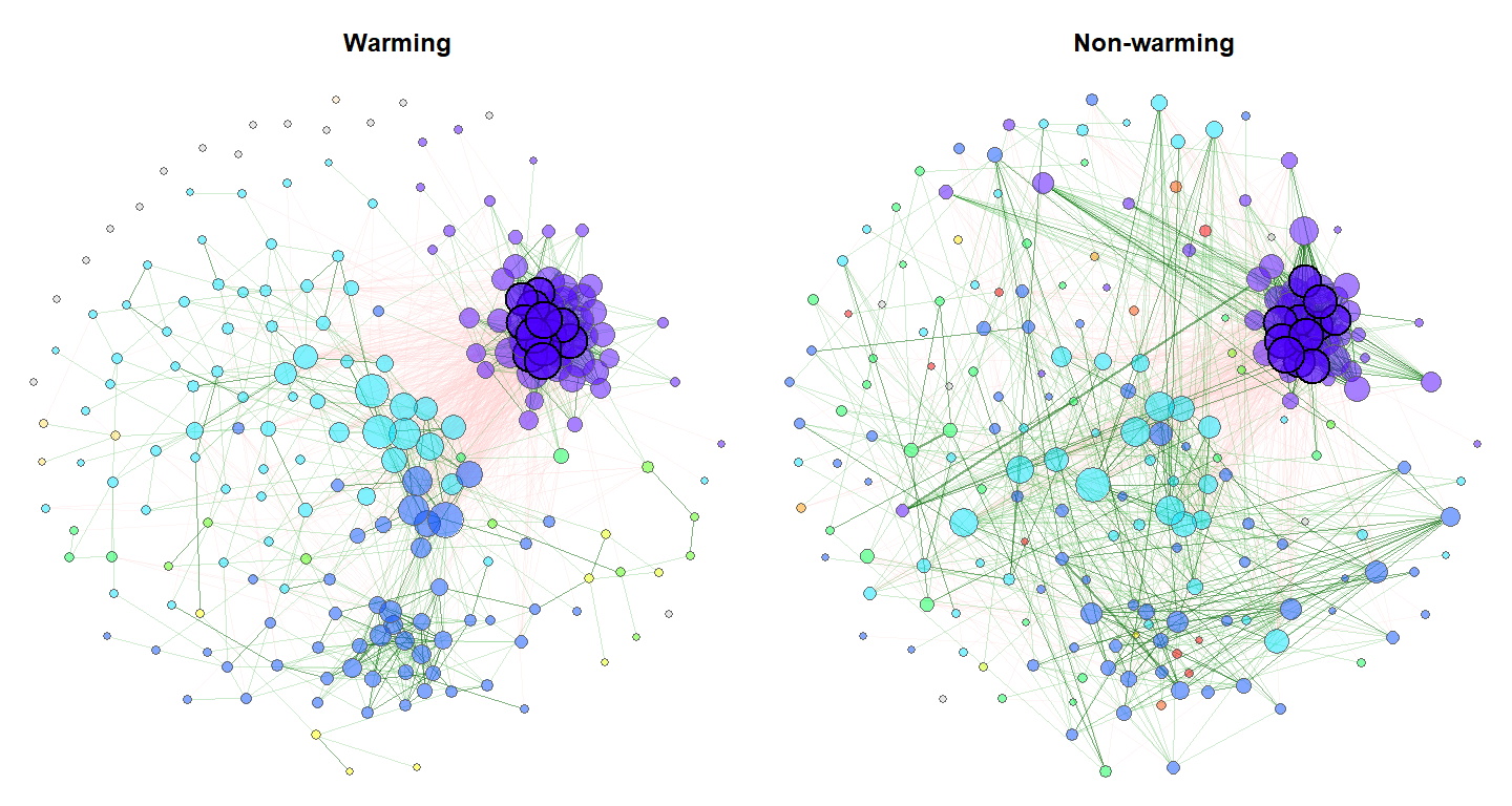
Exemplary network comparison using soil microbiome data (‘soilrep’ data from phyloseq package). Microbial associations are compared between the two experimantal settings ‘warming’ and ‘non-warming’ using the same layout (determines node positions) in both groups.
Here is an overview of methods available for network construction, together with some information on the implementation in R.
Association measures:
- Pearson coefficient
(
cor()fromstatspackage) - Spearman coefficient
(
cor()fromstatspackage) - Biweight Midcorrelation
bicor()fromWGCNApackage - SparCC (own implementation in C++ based on r-sparcc)
- CCLasso (R script on GitHub)
- CCREPE
(
ccrepepackage) - SpiecEasi (
SpiecEasipackage) - SPRING (
SPRINGpackage) - gCoda (R script on GitHub)
- propr
(
proprpackage)
Dissimilarity measures:
- Euclidean distance
(
vegdist()fromveganpackage) - Bray-Curtis dissimilarity
(
vegdist()fromveganpackage) - Kullback-Leibler divergence (KLD)
(
KLD()fromLaplacesDemonpackage) - Jeffrey divergence (own code using
KLD()fromLaplacesDemonpackage) - Jensen-Shannon divergence (own code using
KLD()fromLaplacesDemonpackage) - Compositional KLD (own implementation following [Martín-Fernández et al., 1999])
- Aitchison distance
(
vegdist()andcenLR()fromrobCompositionspackage)
Methods for zero replacement:
- Adding unit pseudo counts
- Multiplicative replacement
(
multReplfromzCompositionspackage) - Modified EM alr-algorithm
(
lrEMfromzCompositionspackage) - Bayesian-multiplicative replacement
(
cmultReplfromzCompositionspackage)
Normalization methods:
- Total Sum Scaling (TSS) (own implementation)
- Cumulative Sum Scaling (CSS) (
cumNormMatfrommetagenomeSeqpackage) - Common Sum Scaling (COM) (own implementation)
- Rarefying (
rrarefyfromveganpackage) - Variance Stabilizing Transformation (VST)
(
varianceStabilizingTransformationfromDESeq2package) - Centered log-ratio (clr) transformation
(
cenLR()fromrobCompositionspackage))
TSS, CSS, COM, VST, and the clr transformation are described in [Badri et al., 2020].
#install.packages("devtools")

devtools::install_github("stefpeschel/NetCoMi", dependencies = TRUE,
                         repos = c("https://cloud.r-project.org/",
                                   BiocManager::repositories()))
If there are any errors during installation, please install the missing dependencies manually.
We use the American Gut data from
SpiecEasi package to look at
some examples of how NetCoMi is applied. The main functions of
NetCoMi are netConstruct() for network construction, netAnalyze()
for network analysis, and netCompare() for network comparison. As you
will see in the following, these three functions must be executed in the
aforementioned order. A further function is diffnet() for constructing
a differential association network. diffnet() must be applied to the
object returned from netConstruct().
First of all, we load NetCoMi and the data from American Gut Project
(provided by SpiecEasi, which
is automatically loaded together with NetCoMi).
library(NetCoMi)
data("amgut1.filt")
data("amgut2.filt.phy")
We construct a single association network using the SPIEC-EASI approach
for estimating associations (conditional dependence) between OTUs.
Additional arguments are passed to spiec.easi() via measurePar.
nlambda and rep.num are set to 20 for a decreased execution time,
but should be higher for real data.
Normalization as well as zero handling is performed internally in
spiec.easi().
net_single <- netConstruct(amgut1.filt, verbose = 3,
                           measure = "spieceasi",
                           measurePar = list(method = "mb",
                                             nlambda=20,
                                             pulsar.params=list(rep.num=20)),
                           normMethod = "none", zeroMethod = "none",
                           sparsMethod = "none", seed = 123456)
## 0 samples removed.
## 0 taxa removed.
## 127 taxa and 289 samples remaining.
##
## Calculate 'spieceasi' associations ...
## Applying data transformations...
## Selecting model with pulsar using stars...
## Fitting final estimate with mb...
## done
## Done.
Analyze the constructed network
Clusters are identified using greedy modularity optimization (by
cluster_fast_greedy() from igraph package).
props_single <- netAnalyze(net_single, clustMethod = "cluster_fast_greedy")Visualize the network
We use the determined clusters as node colors and scale the node sizes according to the node’s eigenvector centrality.
# help page
?plot.microNetPropsplot(props_single, nodeColor = "cluster", nodeSize = "eigenvector")Let’s construct another network using Pearson’s correlation coefficient as association measure. Since Pearson correlations may lead to compositional effects when applied to sequencing data, we use the clr transformation as normalization method. Zero treatment is necessary if the counts are clr transformed. Student’s t-test is used as sparsification method, so that only OTUs with a correlation significantly different from zero are connected.
net_single2 <- netConstruct(amgut1.filt, verbose = 0,
                            measure = "pearson",
                            normMethod = "clr", zeroMethod = "multRepl",
                            sparsMethod = "t-test", adjust = "lfdr")

props_single2 <- netAnalyze(net_single2, clustMethod = "cluster_fast_greedy")

plot(props_single2, nodeColor = "cluster", nodeSize = "eigenvector")Now let’s look how two networks are compared using NetCoMi.
We use ‘SEASONAL_ALLERGIES’, which is part of the phyloseq object, as
group variable. The metagMisc
package offers a function for splitting phyloseq objects according to a
variable. The two resulting phyloseq objects (we ignore the group
‘None’) can directly be passed to NetCoMi.
We select the 50 nodes with highest variance to receive smaller networks.
# devtools::install_github("vmikk/metagMisc")

amgut_split <- metagMisc::phyloseq_sep_variable(amgut2.filt.phy,
                                                "SEASONAL_ALLERGIES")

net_season <- netConstruct(amgut_split$no, amgut_split$yes, verbose = 2,
                           filtTax = "highestVar",
                           filtTaxPar = list(highestVar = 50),
                           measure = "spieceasi",
                           measurePar = list(method = "mb",
                                             nlambda=20,
                                             pulsar.params=list(rep.num=20)),
                           normMethod = "none", zeroMethod = "none",
                           sparsMethod = "none", seed = 123456)
## Data filtering ...
## 0 samples removed in data set 1.
## 0 samples removed in data set 2.
## 95 taxa removed in each data set.
## 1 rows with zero sum removed.
## 1 rows with zero sum removed in data set 2.
## 43 taxa and 162 samples remaining in data set 1.
## 43 taxa and 120 samples remaining in data set 2.
##
## Calculate 'spieceasi' associations ... Done.
##
## Calculate associations for group 2 ... Done.
Alternatively, a group vector could be passed to group, according to
which the data set is split into two groups.
# netConstruct expects samples in rows
countMat <- t(amgut2.filt.phy@otu_table@.Data)
group_vec <- phyloseq::get_variable(amgut2.filt.phy, "SEASONAL_ALLERGIES")

# select the two groups of interest
sel <- which(group_vec %in% c("no", "yes"))
group_vec <- group_vec[sel]
countMat <- countMat[sel, ]

net_season <- netConstruct(countMat, group = group_vec, verbose = 0,
                           filtTax = "highestVar",
                           filtTaxPar = list(highestVar = 50),
                           measure = "spieceasi",
                           measurePar = list(method = "mb",
                                             nlambda=20,
                                             pulsar.params=list(rep.num=20)),
                           normMethod = "none", zeroMethod = "none",
                           sparsMethod = "none", seed = 123456)
Analyze and plot the networks
The object returned from netConstruct() containing both networks is
again passed to netAnalyze(). Network properties are computed for both
networks simultaneously.
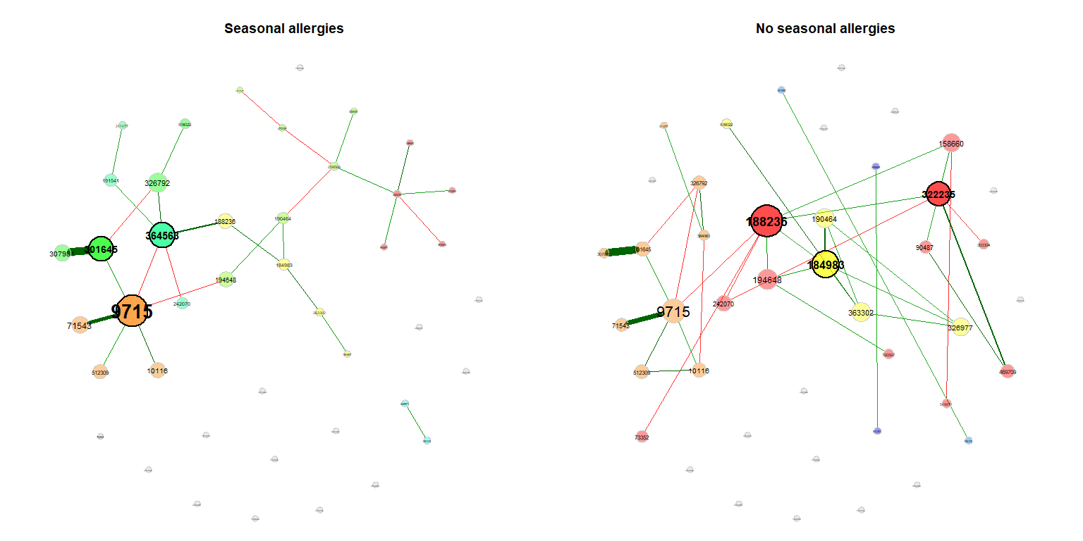
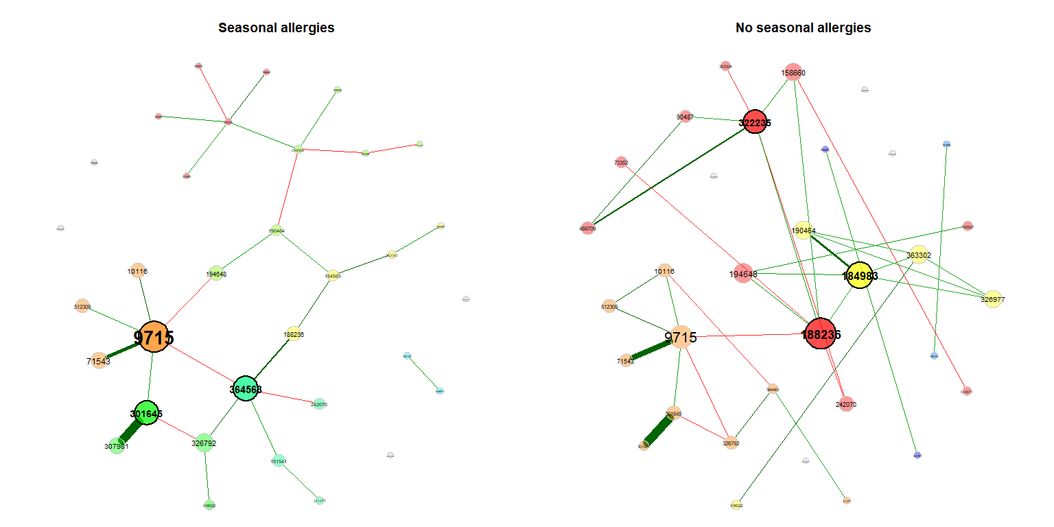
For visualization, we use the same layout (the Fruchterman & Reingold layout) in both groups. In this case, the layout is computed for the left network and adopted to the right one.
props_season <- netAnalyze(net_season, clustMethod = "cluster_fast_greedy")

plot(props_season, sameLayout = TRUE, layoutGroup = 1,
     nodeSize = "eigenvector", cexNodes = 1.5, cexLabels = 1.8,
     groupNames = c("Seasonal allergies", "No seasonal allergies"))
Single nodes can be removed in order to improve readability (if the same layout is used in both groups, only nodes being unconnected in both networks are removed).
plot(props_season, rmSingles = "inboth", sameLayout = TRUE, layoutGroup = 1,
     nodeSize = "eigenvector", cexNodes = 1.5, cexLabels = 1.8,
     groupNames = c("Seasonal allergies", "No seasonal allergies"))
Compare the networks quantitatively
Since execution time is considerably increased if permutation tests are
performed, we set the permTest parameter to FALSE.
comp_season <- netCompare(props_season, permTest = FALSE, verbose = FALSE)It can be chosen, which centrality measures the summary should contain.
summary(comp_season, showCentr = c("degree", "eigen"), numbTaxa = 5)##
## Comparison of Network Properties
## ----------------------------------
##
## CALL:
## netCompare(x = props_season, permTest = FALSE, verbose = FALSE)
##
##
## Jaccard index (similarity betw. sets of most central nodes):
## `````````````
## Jacc P(<=Jacc) P(>=Jacc)
## degree 0.300 0.5592643 0.7008586
## betweenness centr. 0.538 0.9653452 0.1035392
## closeness centr. 0.467 0.9117684 0.2030389
## eigenvec. centr. 0.222 0.2310724 0.8983349
## hub taxa 0.000 0.0877915 . 1.0000000
## -----
## Jaccard index ranges from 0 (compl. different) to 1 (sets equal)
##
##
## Global network properties:
## ``````````````````````````
## group '1' group '2' difference
## average path length 2.551 1.982 0.569
## clustering coeff. 0.000 0.316 0.316
## modularity 0.597 0.601 0.005
## vertex connectivity 0.000 0.000 0.000
## edge connectivity 0.000 0.000 0.000
## edge density 0.032 0.040 0.008
##
##
## Adjusted Rand index (similarity betw. clusterings):
## ```````````````````
## ARI p-value
## 0.253 0
## -----
## ARI in [-1,1] with ARI=1: perfect agreement betw. clusterings,
## ARI=0: expected for two random clusterings
## p-value: two-tailed test with null hypothesis ARI=0
##
##
## Centrality measures (sorted by decreasing diff.):
## ````````````````````
## Degree:
## group '1' group '2' difference
## 188236 0.048 0.167 0.119
## 326977 0.000 0.071 0.071
## 259569 0.095 0.024 0.071
## 469709 0.000 0.048 0.048
## 158660 0.024 0.071 0.048
##
## Eigenvector centrality:
## group '1' group '2' difference
## 322235 0.058 0.704 0.646
## 188236 0.359 1.000 0.641
## 184983 0.227 0.819 0.592
## 364563 0.756 0.178 0.578
## 326977 0.000 0.470 0.470
##
## --------------------------------------------------------
## Significance codes: ***: 0.001, **: 0.01, *: 0.05, .: 0.1
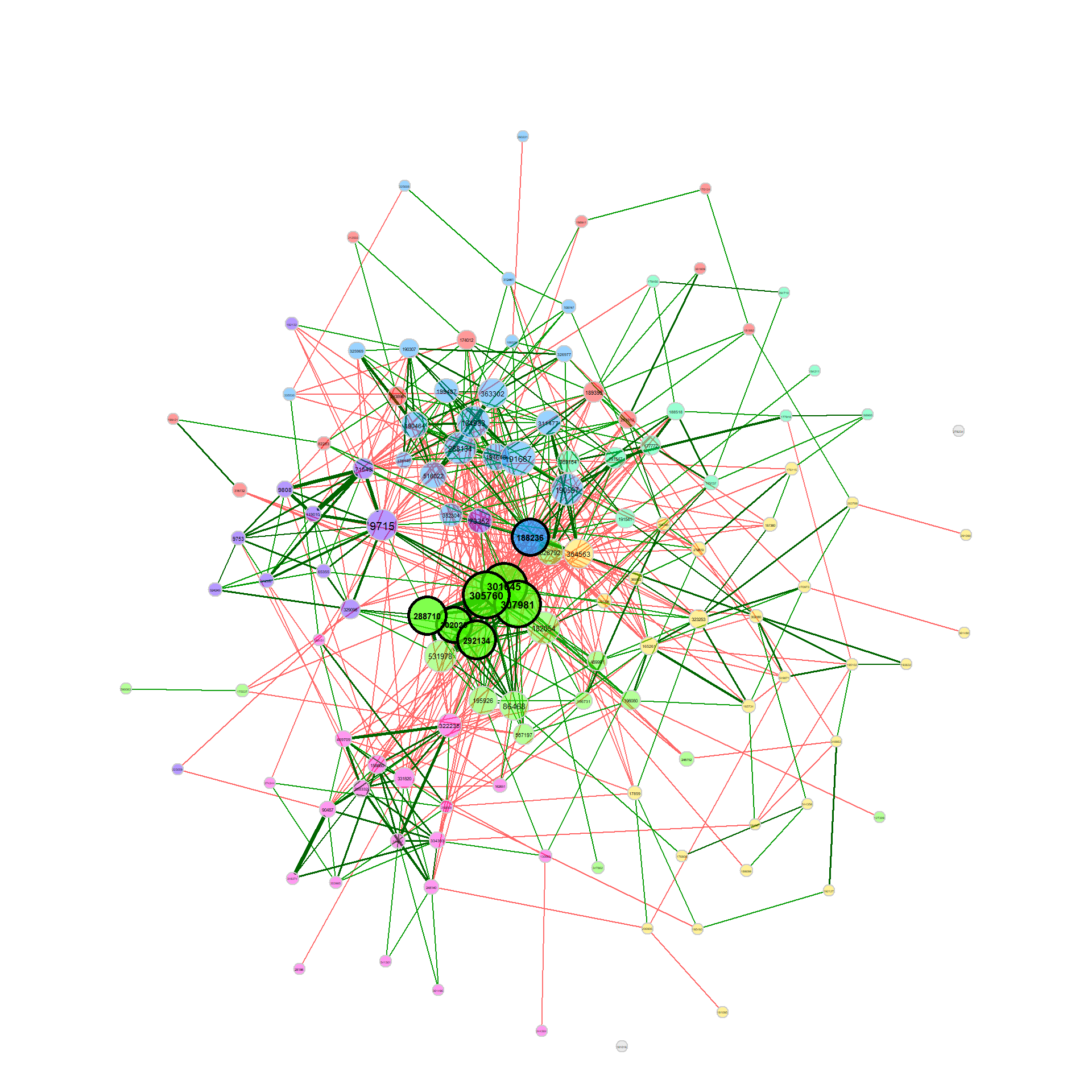
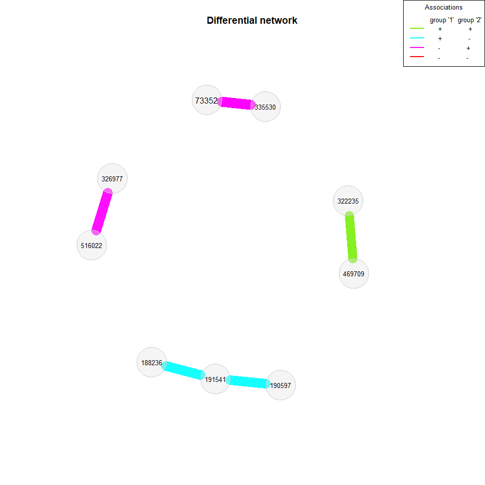
We now build a differential association network, where two nodes are connected if they are differentially associated between the two groups. We again apply Pearson’s correlations to the clr transformed data, but this time a threshold is used as sparsification method so that two OTUs are connected if their absolute correlation is above 0.3.
Fisher’s z-test is used for identifying differentially correlated OTUs, which are connected in the network.
net_season2 <- netConstruct(amgut_split$no, amgut_split$yes, verbose = 0,
                           filtTax = "highestVar",
                           filtTaxPar = list(highestVar = 50),
                           measure = "pearson", normMethod = "clr",
                           sparsMethod = "threshold", thresh = 0.3)

diff_season2 <- diffnet(net_season2, diffMethod = "fisherTest", adjust = "lfdr")
## Adjust for multiple testing using 'lfdr' ...
## Execute fdrtool() ...
## Step 1... determine cutoff point
## Step 2... estimate parameters of null distribution and eta0
## Step 3... compute p-values and estimate empirical PDF/CDF
## Step 4... compute q-values and local fdr
## Done.
<<<<<<< Updated upstream
plot(diff_season2, cexNodes = 0.8, cexLegend = 0.8, mar = c(7,7,7,10))
=======
plot(diff_season2, mar = c(2,1,7,7))
>>>>>>> Stashed changes
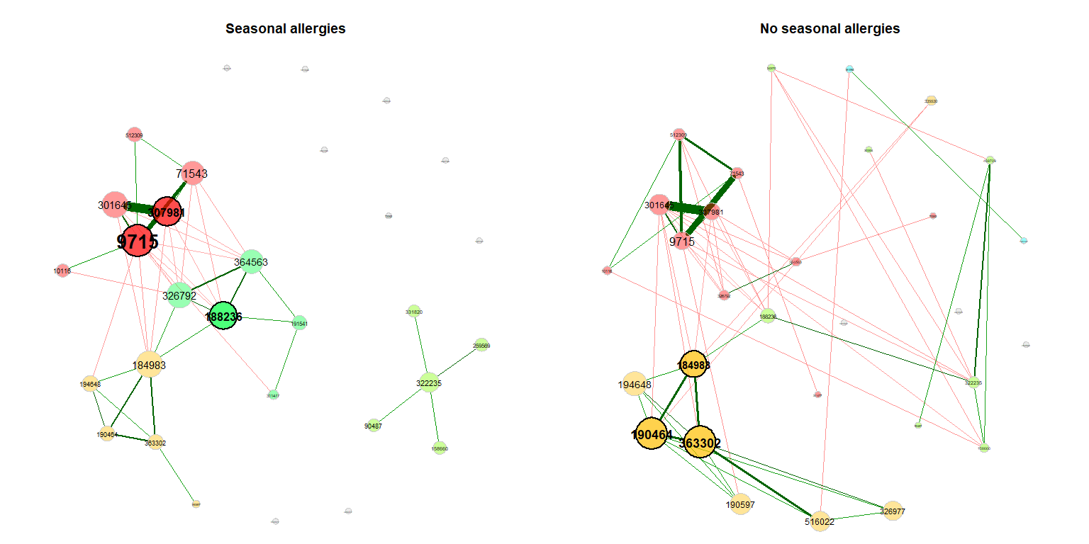
We also take a look at the association networks belonging to the differential network.
props_season2 <- netAnalyze(net_season2, clustMethod = "cluster_fast_greedy")

plot(props_season2, rmSingles = "inboth", sameLayout = TRUE, layoutGroup = 1,
     shortenLabels = "intelligent", nodeSize = "eigenvector",
     cexNodes = 1.5, cexLabels = 1.8,
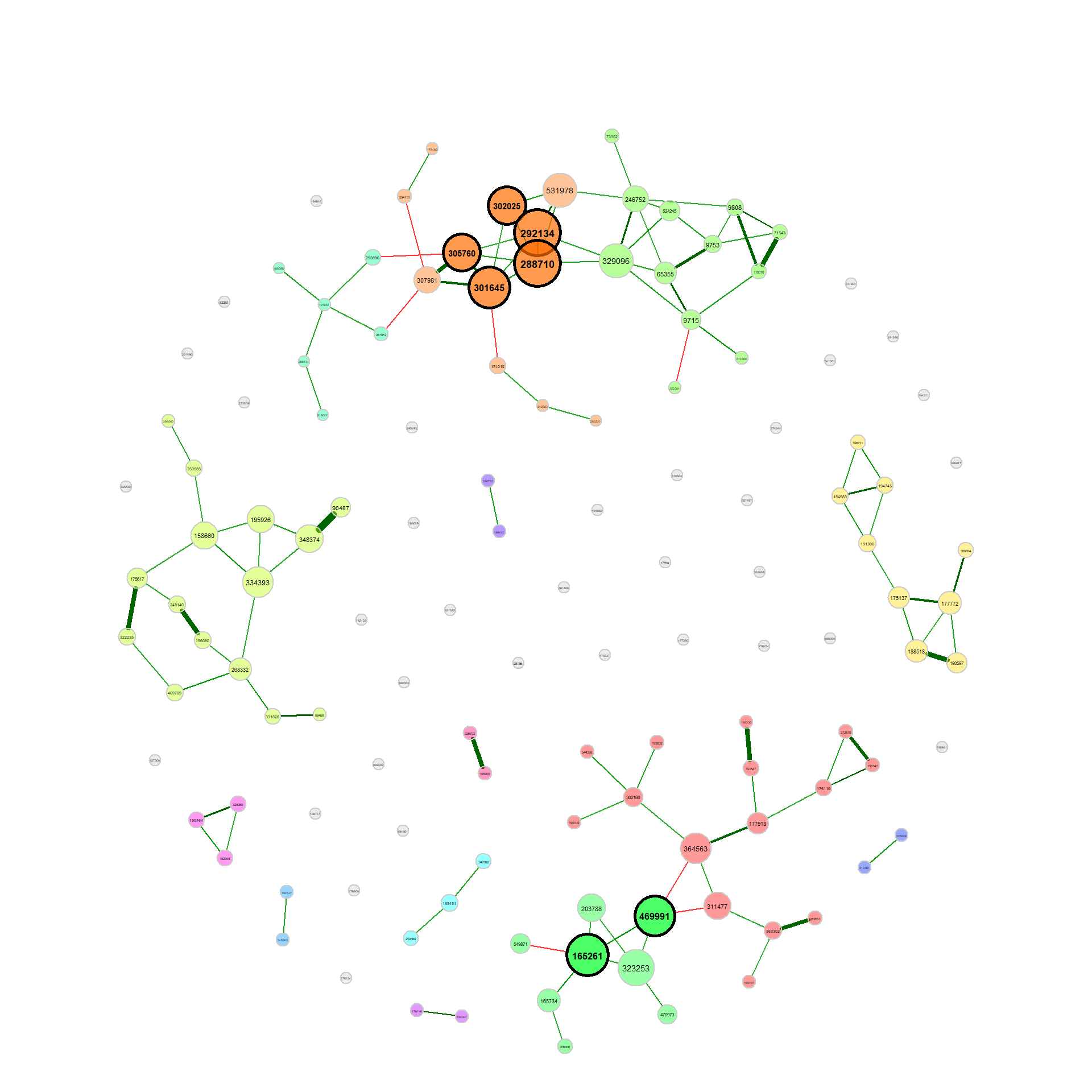
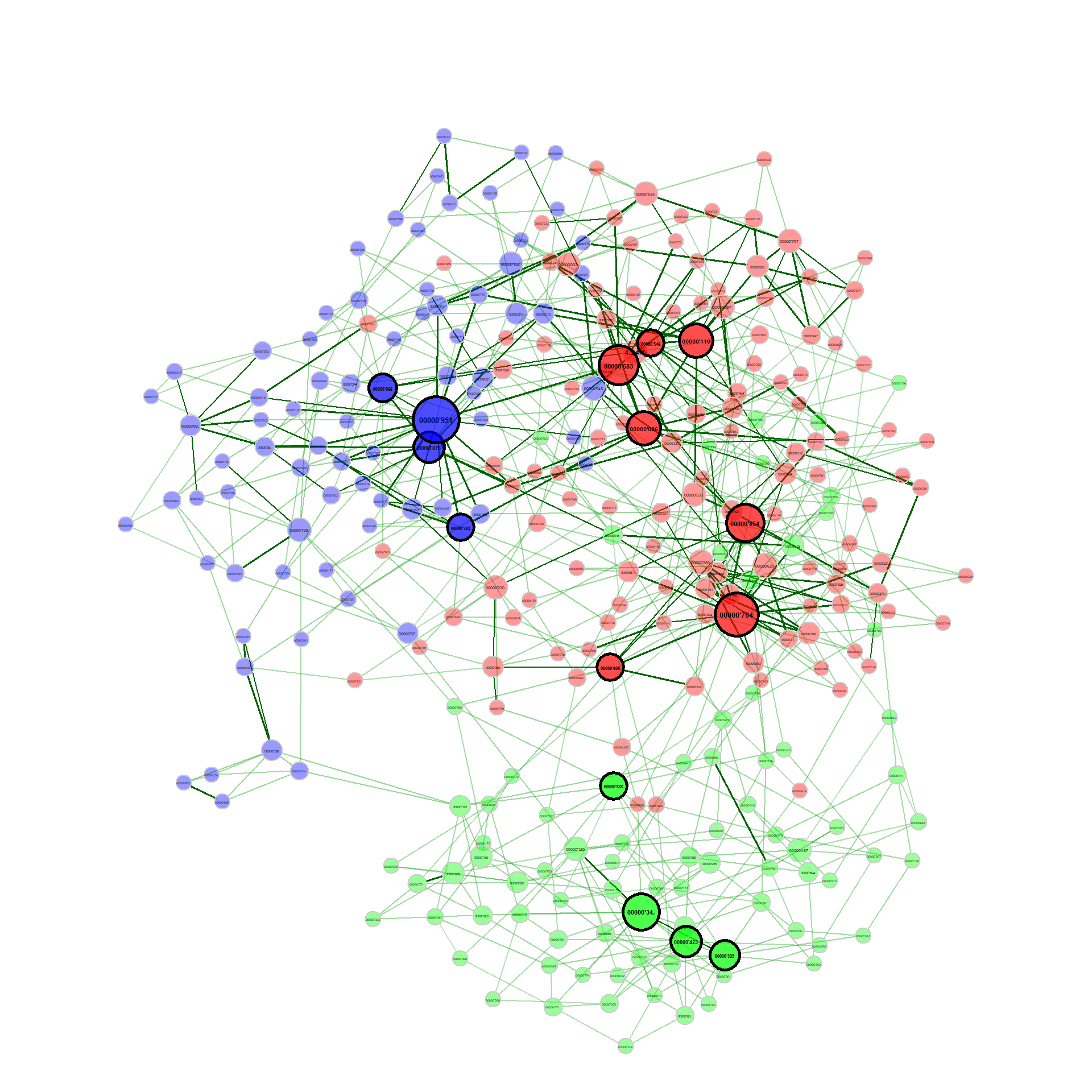
groupNames = c("Seasonal allergies", "No seasonal allergies"))If a dissimilarity measure is used for network construction, nodes are subjects instead of OTUs. The estimated dissimilarities are transformed to similarities, which are used as edge weights so that subjects with a similar microbial composition are placed close together in the network plot.
We construct a single network using Aitchison’s distance being suitable for the application on compositional data.
Since the Aitchison distance is based on the clr-transformation, zeros in the data need to be replaced.
The network is sparsified using the k-nearest neighbor (knn) algorithm.
net_aitchison <- netConstruct(amgut1.filt, verbose = 0,
                              filtTax = "highestFreq",
                              filtTaxPar = list(highestFreq = 100),
                              measure = "aitchison",
                              zeroMethod = "multRepl",
                              sparsMethod = "knn", kNeighbor = 3)
For cluster detection, we use hierarchical clustering with average
linkage. Internally, k=3 is passed to
cutree()
from stats package so that the tree is cut into 3 clusters.
props_aitchison <- netAnalyze(net_aitchison,
                              clustMethod = "hierarchical",
                              clustPar = list(method = "average", k = 3),
                              hubPar = "degree")

plot(props_aitchison, nodeColor = "cluster", nodeSize = "degree",
edgeTranspLow = 60)Here is the code to produce the network plot shown at the beginning.
data("soilrep")
soil_warm <- metagMisc::phyloseq_sep_variable(soilrep, "warmed")

net_seas_p <- netConstruct(soil_warm$yes, soil_warm$no,
                         filtTax = "highestVar",
                         filtTaxPar = list(highestVar = 500),
                         verbose = 3, measure = "pearson",
                         zeroMethod = "pseudo",
                         normMethod = "clr")

netprops1 <- netAnalyze(net_seas_p, clustMethod = "cluster_fast_greedy")

nclust <- as.numeric(max(names(table(netprops1$clustering$clust1))))
col <- topo.colors(nclust)

plot(netprops1, sameLayout = TRUE, layoutGroup = 1, colorVec = col,
     borderCol = "gray40", nodeSize = "degree", cexNodes = 35,
     nodeSizeSpread = 0.1, edgeTranspLow = 80, edgeTranspHigh = 50,
     groupNames = c("Warming", "Non-warming"), showTitle = TRUE, cexTitle = 1.5,
     mar = c(1,1,3,1), repulsion = 0.9, labels = FALSE, rmSingles = "inboth",
     nodeFilter = "clustMin", nodeFilterPar = 10,
nodeTransp = 50, hubTransp = 30)[Martín-Fernández et al., 1999] Josep A Martín-Fernández, Mark J Bren, Carles Barceló-Vidal, and Vera Pawlowsky-Glahn (1999). A measure of difference for compositional data based on measures of divergence. Lippard, Næss, and Sinding-Larsen, 211-216.)
[Badri et al., 2020] Michelle Badri, Zachary D. Kurtz, Richard Bonneau, and Christian L. Müller (2020). Shrinkage improves estimation of microbial associations under different normalization methods. bioRxiv, doi: 10.1101/406264.
