DINO configuration

A DIabatic NeverwOrld2 in NEMO. This repository contains the source for the NEMO configurartion DINO.

Grid

Horizontal discretization

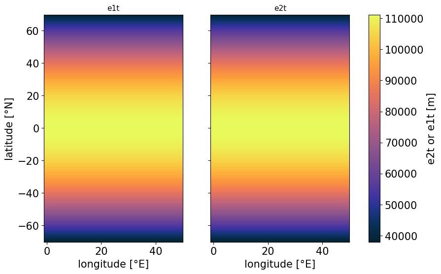
DINO is solved on a sphere and discretized by a horizontally isotropic mercator grid. Therefore, the grid-spacing in latitudinal direction decreases towards the poles.

We compute longitude at T-points as $$ \begin{equation*} \lambda(i) = \lambda_{0} + \Delta \lambda * i \end{equation*} $$

where $i \in \left[ 1, I \right]$ and latitude at T-points as $$ \begin{equation*} \phi(j) = \frac{180}{\pi} * \arcsin ( \tanh( \Delta \lambda \frac{\pi}{180} * j) ) \end{equation*} $$

where $j \in \left[ 1, J \right]$.
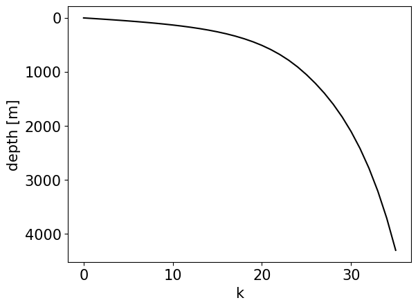
The prognostic variables are staggered on an Arakawa C-grid. $I$ and $J$ are chosen to span a domain of 50° from eastern to western boundary and approximately 70° (not exactly, due to the mercator projection in (2)) from equator to both northern and southern boundary. In the following we show an example of the resulting grid spacing along $y$ (e2t) and $x$ (e1t) in meters for $\Delta \lambda = 1.0$:

Vertical discretization

Since this commit DINO has the option for a full step z* vertical coordinate. It follows exactly the same stretching function as the hybrid sigma-z coordinate, but assuming a flat bottom:
With $$ \begin{align*} a_0 &= \left( dz_{min} - \frac{H - h_{co}}{K - 1 - k_{const}}\right)/ \left(\tanh{\left(\frac{1 - k_{th}}{a_{cr}}\right)} - a_{cr} \cdot \frac{\ln{\left( \cosh{\left(\frac{K - k_{const} - k_{th}}{a_{cr}}\right)}\right)} - \ln{\left(\cosh{\left(\frac{1 - k_{th}}{a_{cr}}\right)}\right)}}{K - 1 - k_{const}}\right) \ a_1 &= dz_{min} - a_0 \cdot \tanh{\left(\frac{1 - k_{th}}{a_{cr}}\right)} \

a_2 &= -a_1 - a_0 \cdot a_{cr} \cdot \ln{\left(\cosh{\left(\frac{1 - k_{th}}{a_{cr}}\right)}\right)}

\end{align*}

We compute the depth at T-points $$ z_t = a_2 + a_1 \cdot k_t + a_0 \cdot a_{cr} \cdot \ln{\left(\cosh{\left(\frac{k_w - k_{th}}{a_{cr}}\right)}\right)} + h_{co}, $$ where

$$ k_t = k - k_{const} + 0.5 $$

and depth at W-points $$ z_w = a_2 + a_1 \cdot k_w + a_0 \cdot a_{cr} \cdot \ln{\left(\cosh{\left(\frac{k_t - k_{th}}{a_{cr}}\right)}\right)} + h_{co}, $$

where

$$ k_w = k - k_{const} $$

This is done once for the top z-level using the parameters $$ \begin{align*} &H = 4000 &&: \text{Depth of the bottom [meters]} \ &dz_{min} = 10 &&: \text{Value of e3 at the connection point [meters]} \ &h_{co} = 0 &&: \text{Depth of the connection between z- and s-coordinat es [meters]} \ &k_{th} = 35 &&: \text{Position of the inflexion point} \ &k_{const} = 0 &&: \text{Index of last level with z-coordinates} \ &a_{cr} = 10.5 &&: \text{Slope of the tanh function}, \end{align*} $$

and then repeated for the bottom "sigma"-level with adapted diagnosed parameters

$$ \begin{align*} &k_{const} &&= argmin(abs(z_w - 1000m) &&: \text{Index of last level with z-coordinates} \\ &dz_{min} &&= diff(z_t)[k_{const}] &&: \text{Value of e3 at the connection point [meters]} \\ &h_{co} &&= z_w[k_{const}] &&: \text{Depth of the connection between z- and s-coordinat es [meters]} \\ \end{align*} $$

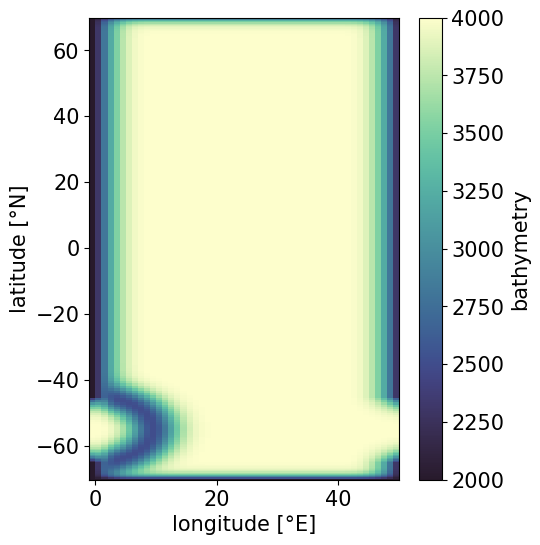
The vertical index $k \in \left[ 1, K \right]$ with $K=36$. The resulting depth level over k are shown in the following:

Bathymetry

The domain is closed everywhere except a periodic re-entrant channel between $45°S$ and $65°S$. Above $2000m$ depth the domain is bounded by vertical walls, below a tapered exponential defines the slopes. A semi-circular sill with a Gaussian shape introduces a pressure gradient in the channel, similar to the Neverworld2 configuration. The exact implementation is demonstrated in DinoConfiguration.get_bathymetry() and DinoConfiguration.add_gaussian_ring(). In the following we show the resulting bathymetry for the standard configuration:

Equation of State (EOS)

We follow the simplified EOS from Roquet et al. (2015)

$$ \begin{equation*} \rho(T,S,p) = \rho_{0} - \left( a_{0} + \frac{1}{2} C_{b} T_{a} + T_{h} p \right) T_{a} + b_{0} S_{a} \end{equation*} $$

where $$ \begin{align*} T_{a} &= T - 10°C \ S_{a} &= S - 35 , \text{g} , \text{kg}^{-1} \end{align*} $$

using the parameters:

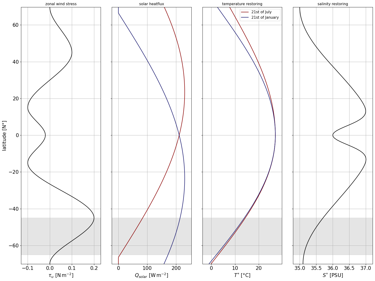
$$ \begin{align*} &\rho_{0} = 1028 &&: \text{reference density } [\text{kg} , \text{m}^{-3}] \\ &a_{0} = 0.1655 &&: \text{thermal expansion } [\text{kg} , \text{m}^{-3} , \text{K}^{-1}] \\ &b_{0} = 0.7655 &&: \text{haline expansion } [\text{kg}^{2} , \text{m}^{-3} , \text{g}^{-1}] \\ &C_{b} = 9.9 \times 10^{-3} &&: \text{thermal cabbeling } [\text{kg} , \text{m}^{-3} , \text{K}^{-2}] \\ &T_{h} = 2.4775 \times 10^{-5} &&: \text{thermobaricity } [\text{kg}^{-3} , \text{dbar}^{-1} , \text{K}^{-1}] \end{align*} $$

Surface Boundary Conditions

We need to define surface boundary conditions for all prognostic variables, namely $U$, $V$, $T$, and $S$. Regarding momentum we follow Marques et al 2020 with a purely zonal wind stress profile constructed with a piecewise cubic interpolation between fixed values of latitude.

Temperature $T$ and salinity $S$ are restored towards meridional profiles, defined through

$$ T^{}(\phi) = T^{}{n/s} + \left( T^{*}{eq} - T^{*}_{n/s} \right) , \sin(\pi , \frac{\phi + \phi_n}{\phi_n - \phi_s}) $$

and

$$ S^{}(\phi) = S^{}{n/s} + \left( S^{*}{eq} - S^{*}_{n/s} \right) , \left(1 + \cos(\frac{2 , \pi , \phi }{\phi_n - \phi_s})\right) / 2 - 1.25 , e^{- \phi^{2} / 7.5^{2}} $$

where the subscript $(...)_{n/s}$ denotes the value at the northern or southern boundary, when $\phi < 0$ or $\phi > 0$. The restoring values for southern, northern boundary and equator are

$$ \begin{align*} &T^{}_{s} = -0.5°C, &&T^{}{n} = -5.0°C, &&T^{*}{eq} = 27.0°C \ &S^{}_{s} = 35.1 PSU, &&S^{}{n} = 35.0 PSU, &&S^{*}{eq} = 37.25 PSU \ \end{align*}. $$

The salinity restoring stays constant throughout the simulation, while a seasonal cosine of magnitude $3.0°C$ (at $T^{}_{n}$) and $0.5°C$ (at $T^{}_{s}$) is applied to the boundary values of the temperature restoring. The maximum/minimum restoring lags one month after the respective minimum/maximum in solar radiation. All meridional profiles of surface boundary conditions are visualized below.

Shortwave solar radiation is adapted from Caneill et al. 2022 and given by

$$ Q_{solar}(\phi) = 230. , \cos\left( \frac{\pi}{180} , \left[ \phi - 23.5 , \cos(\pi ,\frac{d+189}{180})\right]\right) $$

where d is the day of the year controlling a seasonal cycle in the solar forcing.