ParBayesianOptimization

Installation

You can install the most recent stable version of ParBayesianOptimization from CRAN with:

install.packages("ParBayesianOptimization")

You can also install the most recent development version from github using devtools:

# install.packages("devtools")
devtools::install_github("AnotherSamWilson/ParBayesianOptimization")

Package Process

Machine learning projects will commonly require a user to “tune” a model’s hyperparameters to find a good balance between bias and variance. Several tools are available in a data scientist’s toolbox to handle this task, the most blunt of which is a grid search. A grid search gauges the model performance over a pre-defined set of hyperparameters without regard for past performance. As models increase in complexity and training time, grid searches become unwieldly.

Idealy, we would use the information from prior model evaluations to guide us in our future parameter searches. This is precisely the idea behind Bayesian Optimization, in which our prior response distribution is iteratively updated based on our best guess of where the best parameters are. The ParBayesianOptimization package does exactly this in the following process:

Initial parameter-score pairs are found
Gaussian Process is fit/updated
Numerical methods are used to estimate the best parameter set
New parameter-score pairs are found
Repeat steps 2-4 until some stopping criteria is met

Bayesian Optimization Intuition

As an example, let’s say we are only tuning 1 hyperparameter in an random forest model, the number of trees, within the bounds [1,5000]. We have initialized the process by randomly sampling the scoring function 7 times, and get the following results:

Trees.In.Forest	Score
1	2.00
700	2.43
1865	2.71
2281	2.98
2600	2.54
3000	1.95
4410	1.29

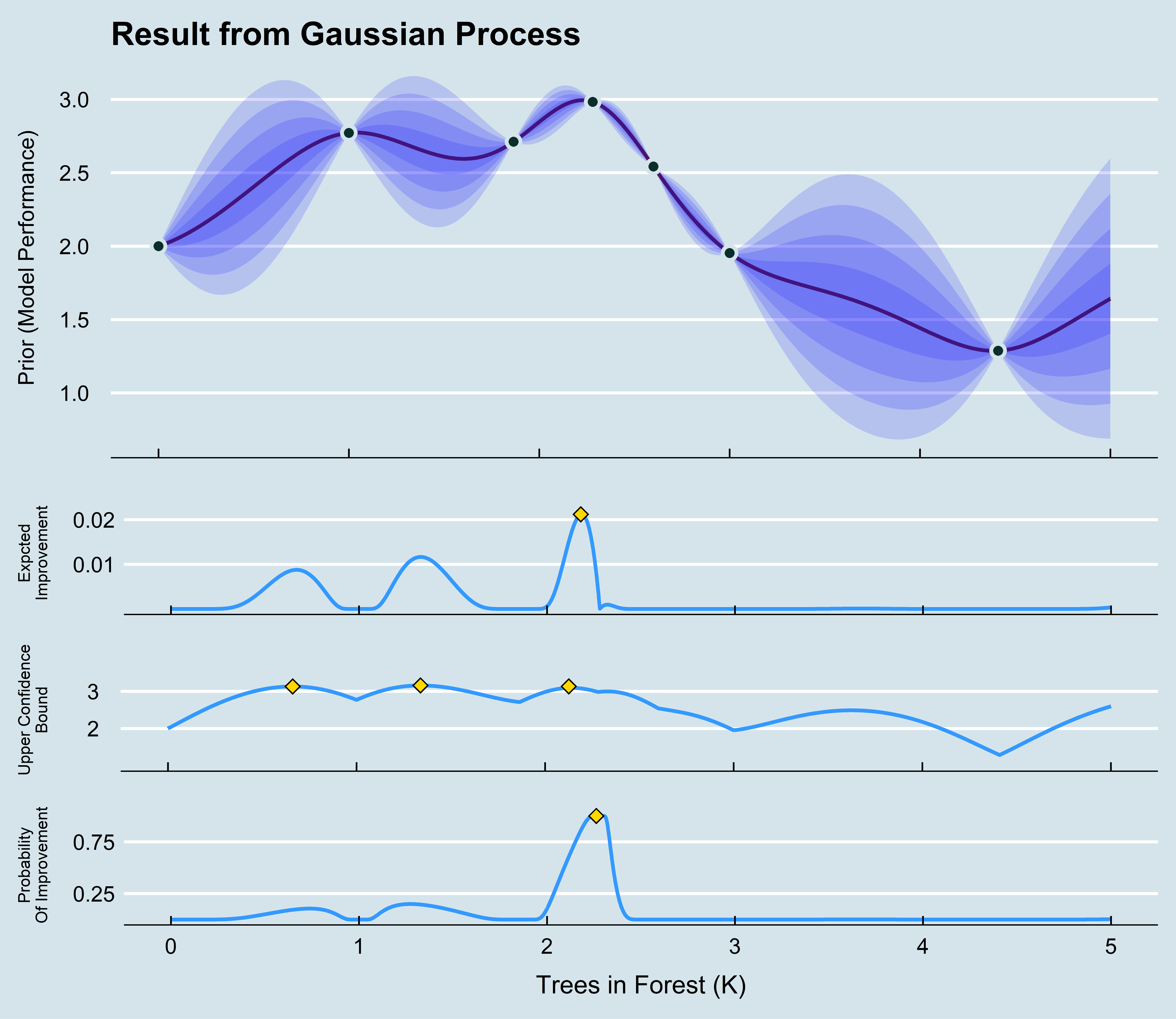
In this example, Score can be generalized to any error metric that we want to maximize (negative RMSE, AUC, etc.). Given these scores, how do we go about determining the best number of trees to try next? As it turns out, Gaussian processes can give us a very good definition for our prior distribution. Fitting a Gaussian process to the data above (indexed by our hyperparameter), we can see the expected value of Score accross our parameter bounds, as well as the uncertainty bands:

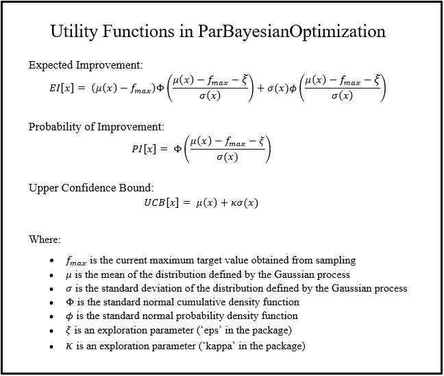
Before we can select our next candidate parameter to run the scoring function on, we need to determine how we define a “good” parameter inside this prior distribution. This is done by maximizing different utility functions within the Gaussian process. There are several functions to choose from:

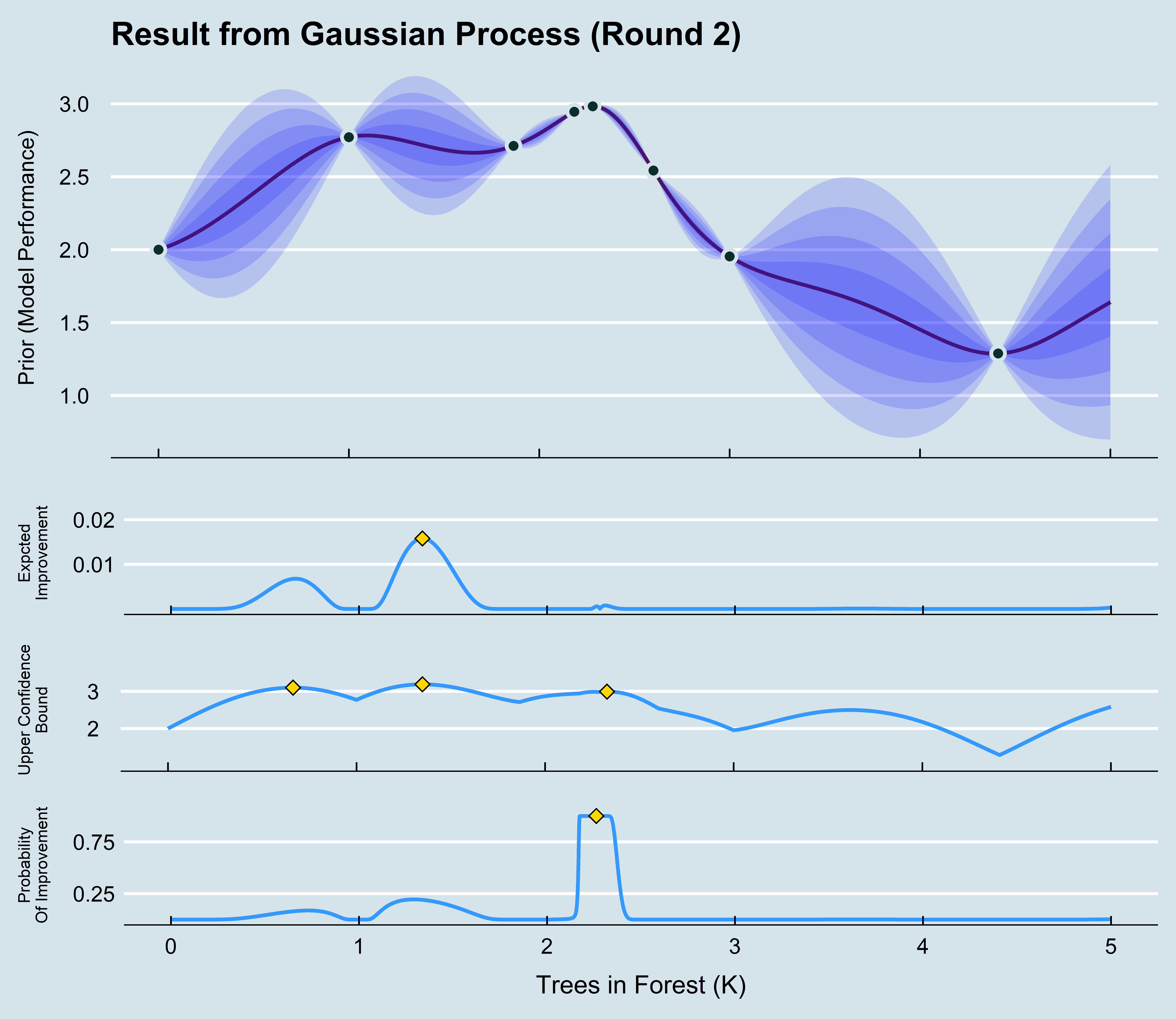
Our expected improvement in the graph above is maximized at ~2180. If we run our process with the new Trees in Forest = 2180, we can update our Gaussian process for a new prediction about which would be best to sample next:

As you can see, our updated gaussian process has a maximum expected improvement at ~ Trees in Forest = 1250. We can continue this process until we are confident that we have selected the best parameter set.

The utility functions that are maximized in this package are defined as follows:

An advanced feature of ParBayesianOptimization, which you can read about in the vignette advancedFeatures, describes how to use the minClusterUtility parameter to search over the different local maximums shown above. For example, in the first chart, we the process would sample all 3 optimums in the Upper Confidence Bound utility. If minClusterUtility is not specified, only the global maximum would be sampled.

Practical Example

In this example, we will be using the agaricus.train dataset provided in the XGBoost package. Here, we load the packages, data, and create a folds object to be used in the scoring function.

library("xgboost")
library("ParBayesianOptimization")
#> Warning: package 'ParBayesianOptimization' was built under R version 3.5.3

data(agaricus.train, package = "xgboost")

Folds <- list(Fold1 = as.integer(seq(1,nrow(agaricus.train$data),by = 3))
            , Fold2 = as.integer(seq(2,nrow(agaricus.train$data),by = 3))
            , Fold3 = as.integer(seq(3,nrow(agaricus.train$data),by = 3)))

Now we need to define the scoring function. This function should, at a minimum, return a list with a Score element, which is the model evaluation metric we want to maximize. We can also retain other pieces of information created by the scoring function by including them as named elements of the returned list. In this case, we want to retain the optimal number of rounds determined by the xgb.cv:

scoringFunction <- function(max_depth, min_child_weight, subsample) {
  
  set.seed(3)

  dtrain <- xgb.DMatrix(agaricus.train$data,label = agaricus.train$label)
  
  Pars <- list( booster = "gbtree"
              , eta = 0.01
              , max_depth = max_depth
              , min_child_weight = min_child_weight
              , subsample = subsample
              , objective = "binary:logistic"
              , eval_metric = "auc")

  xgbcv <- xgb.cv(params = Pars
                , data = dtrain
                , nround = 100
                , folds = Folds
                , prediction = TRUE
                , showsd = TRUE
                , early_stopping_rounds = 5
                , maximize = TRUE
                , verbose = 0)

  return(list(Score = max(xgbcv$evaluation_log$test_auc_mean)
             , nrounds = xgbcv$best_iteration
             )
         )
}

Some other objects we need to define are the bounds, GP kernel and acquisition function.

The bounds will tell our process its search space.
The kernel is passed to the GauPro function GauPro_kernel_model and defines the covariance function.
The acquisition function defines the utility we get from using a certain parameter set.

bounds <- list( max_depth = c(2L, 10L)
              , min_child_weight = c(1L, 100L)
              , subsample = c(0.25, 1))

kern <- "Matern52"

acq <- "ei"

We are now ready to put this all into the BayesianOptimization function.

tNoPar <- system.time(
  ScoreResult <- BayesianOptimization(
      FUN = scoringFunction
    , bounds = bounds
    , initPoints = 4
    , bulkNew = 1
    , nIters = 6
    , kern = kern
    , acq = acq
    , kappa = 2.576
    , verbose = 1
    , parallel = FALSE)
)
#> 
#> Running initial scoring function 4 times in 1 thread(s).
#> 
#> Starting round number 1
#>   1) Fitting Gaussian process...
#>   2) Running local optimum search...
#>   3) Running scoring function 1 times in 1 thread(s)...
#> 
#> Starting round number 2
#>   1) Fitting Gaussian process...
#>   2) Running local optimum search...
#>   3) Running scoring function 1 times in 1 thread(s)...

The console informs us that the process initialized by running scoringFunction 4 times. It then fit a Gaussian process to the parameter-score pairs, found the global optimum of the acquisition function, and ran scoringFunction again. This process continued until we had 10 parameter-score pairs. You can interrogate the ScoreResult object to see the results. As you can see, the process found better parameters after each iteration:

ScoreResult$ScoreDT
#>    Iteration max_depth min_child_weight subsample Elapsed     Score nrounds
#> 1:         0         4               70 0.7666946    0.12 0.9779723       1
#> 2:         0         8               16 0.8835947    1.39 0.9990767      54
#> 3:         0         6               48 0.3199902    0.29 0.9790360      13
#> 4:         0         2               89 0.4694295    0.32 0.9779697      19
#> 5:         1         8               13 0.8989494    1.35 0.9993013      51
#> 6:         2         9               11 0.9174873    1.00 0.9994490      36

ScoreResult$BestPars
#>    Iteration max_depth min_child_weight subsample     Score nrounds elapsedSecs
#> 1:         0         8               16 0.8835947 0.9990767      54      3 secs
#> 2:         1         8               13 0.8989494 0.9993013      51     12 secs
#> 3:         2         9               11 0.9174873 0.9994490      36     22 secs

Running In Parallel

The process that the package uses to run in parallel is explained above. Actually setting the process up to run in parallel is relatively simple, we only need to define two additional parameters in the BayesianOptimization function, export and packages:

exp <- c('agaricus.train','Folds')
pac <- c('xgboost')

We also must register a parallel backend, which we do using the doParallel package. The bulkNew parameter is set to 2 to make full use of the registered cores:

library(doParallel)
#> Loading required package: foreach
#> Loading required package: iterators
#> Loading required package: parallel
cl <- makeCluster(2)
registerDoParallel(cl)

tWithPar <- system.time(
  ScoreResult <- BayesianOptimization(
      FUN = scoringFunction
    , bounds = bounds
    , initPoints = 8
    , bulkNew = 2
    , nIters = 10
    , kern = kern
    , acq = acq
    , kappa = 2.576
    , parallel = TRUE
    , export = exp
    , packages = pac
    , verbose = 0)
)
stopCluster(cl)
registerDoSEQ()

We managed to massively cut the process time by running the process on 2 cores in parallel: