-
https://[Venky to Provide - Update your details here].
-
https://[Gab to Provide - CDW Workshop (Recording)].
-
https://[Gab to Provide - End-to-End Workshop (Recording)].
-
Laptop with a supported OS (Windows 7 not supported) or MacBook.
-
A modern browser - Google Chrome (IE, Firefox, Safari not supported).
Working for an Aircraft Engine company, the company wants to increase competitive advantage in two keyways:
(1) Engineer better, more fault tolerant aircraft engines.
(2) Be proactive in predictive maintenance on engines, and faster discovery-to-fix in new engine designs.
This will be a three-phase plan:
(1) Phase One: Understand how our current engines contribute to airline flight delays and fix for future engines.
(2) Phase Two: Implement an ongoing reporting service to support ongoing engineering efforts to continuously improve engines based on delay data.
(3) Phase Three: Move to real-time analysis to fix things before they break both in engines already sold, and in new engine designs.
To do this, we’re going to build a data warehouse & data lakehouse to create reports that engineers can use to improve our engines. The following people will get to work:
We will dive into this Scenario to show Cloudera Data Warehouse (CDW) is used to enable the Aircraft company to gain competitive advantage - and at the same time it highlights the performance and automation capabilities that help ensure performance is maintained while controlling costs.
The Hands on Labs will take you through how to use the Cloudera Data Warehouse service to quickly explore raw data, create curated versions of the data for simple reporting and dashboarding, and then scale up usage of the curated data by exposing it to more users.
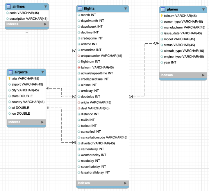
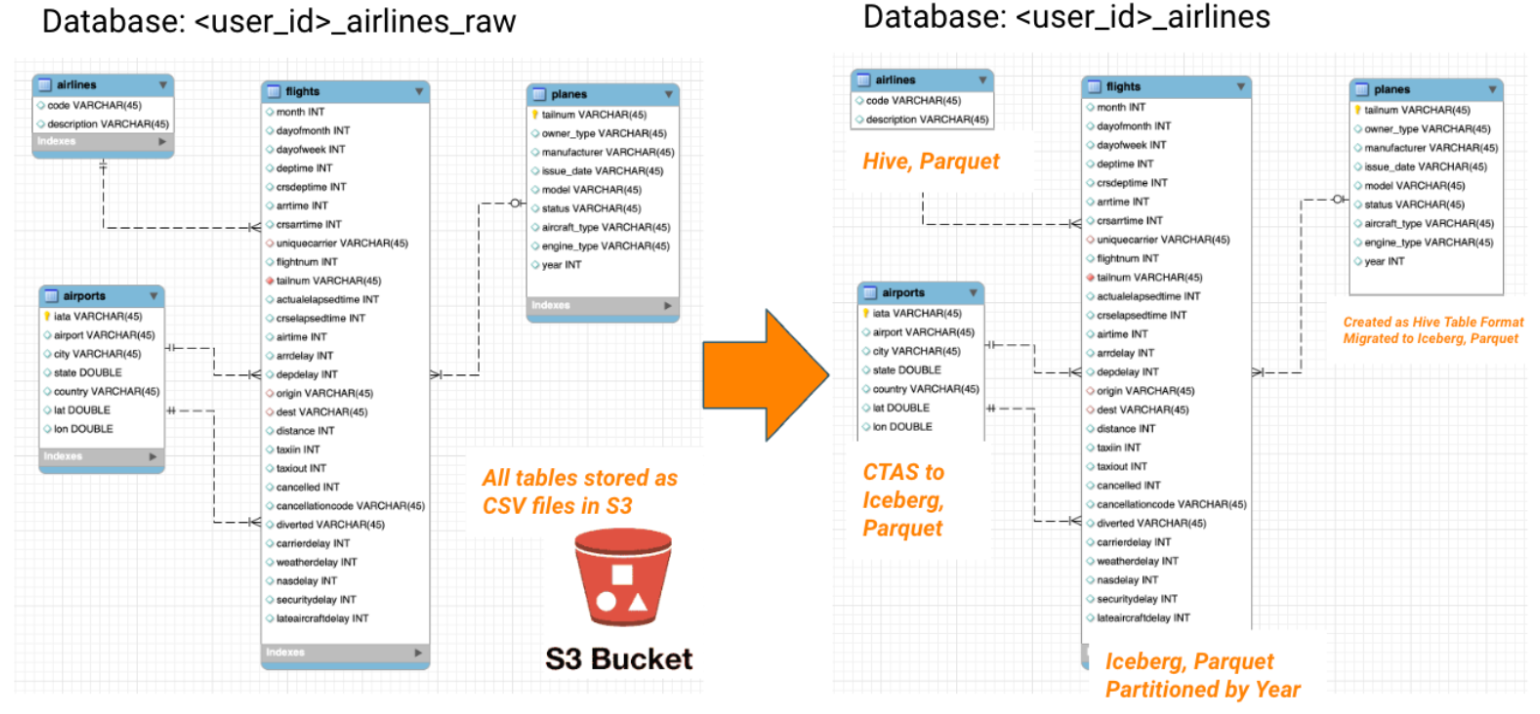
ER - Diagram of the data
(1) Fact Table: flights (86M rows)
(2) Dimension Table: airlines (1.5k rows), airports (3.3k rows) and planes (5k rows)
Below are the high-level steps for what we will be doing in the workshop.
[Step 1 & 2]: General introduction to CDW to get ourselves oriented for the workshop.
(a) As an Admin: Create and enable the BI analyst team with a Virtual Warehouse.
(b) As a BI Analyst:  Get familiar with CDW on CDP and set up our first VW to start working.
(c) As a BI Analyst:  Wrangle our first set of data - sent to us as a series of .csv files exported from “somewhere else”.
(d) As an Admin: Monitor the VW and watch as it scales up and down, suspends, etc.
(e) As a BI Analyst:  Start digging into the data - looking for “needle in a haystack” - running a complex query that will find which engines seem to be correlated to airplane delays for any reason.
[Step 3]: Set it up.
(a) As an Admin: Create and enable the BI analyst team with a Virtual Warehouse.
(b) As a BI Analyst:  Get familiar with CDW on CDP, and set up our first VW to start working.
(c) As a BI Analyst:  Wrangle our first set of data - sent to us as a series of .csv files exported from “somewhere else”.
(d) As an Admin: Monitor the VW and watch as it scales up and down, suspends, etc.
(e) As a BI Analyst:  Start digging into the data - looking for “needle in a haystack” - running a complex query that will find which engines seem to be correlated to airplane delays for any reason.
[Step 4]: Making it better.
(a) As a BI Analyst: Start curating data and building a data lakehouse to improve quality by tweaking data, performance by optimizing schema structures, and ensure reliability and trustworthiness of the data through snapshots, time travel, and rollback.
(b) Create Hive ACID tables and tweak data for consistency (ex: airline name changes - ensure reporting is consistent with the new name to avoid end user confusion, a new airline joins our customer list, make sure they’re tracked for future data collection, etc..).
(c) Migrate Tables to Iceberg (We want snapshot and rollback).
(d) Create new Iceberg tables (we want partitioning).
[Step 5]: Optimizing for production.
(a) Loading more data - change partitioning to maintain performance (NOTE:  Ongoing ELT = CDE?).
(b) Bad data is loaded - use time travel to detect, and rollback to resolve.
(c) Introduce materialized views to support scaling to 1000’s of simultaneous users.
(d) As an admin:  Monitor, report, kill queries that run amock, etc.
[Step 6]: Security & Governance.
(a) Check on the lineage to enable governance/audit.
(b) Row level security to make sure only relevant party can see data.
[Step 7]: Cloudera Data Visualization
(a) Data Modeling for the lakehouse.
(b) Data Visualization for insights.
|
Warning
|
Please make sure that you are working on the browser (Chrome)  in INCOGNITIO MODE in INCOGNITIO MODE  only for the entirety of the workshop. only for the entirety of the workshop. |
Please note the following:
(a) Workshop Login Username: ___ _(Your Instructor would provide this)
(b) Workshop Login Password: ___ _(Your Instructor would provide this)
(c) CDP Workload User (${user_id} or <user_id>): ___ _(Your Instructor would provide this)
(d) CDP Workload Password: ___ (You will set it in Step 1(b) of the workshop)
(e) Hive Virtual Warehouse Name: ___ _(Your Instructor would provide this)
(f) Impala Virtual Warehouse Name: ___ _(Your Instructor would provide this)
In the labs when you see:
${user_id} or <user_id> - this will indicate to use your User (CDP Workload User) as item (c) above.
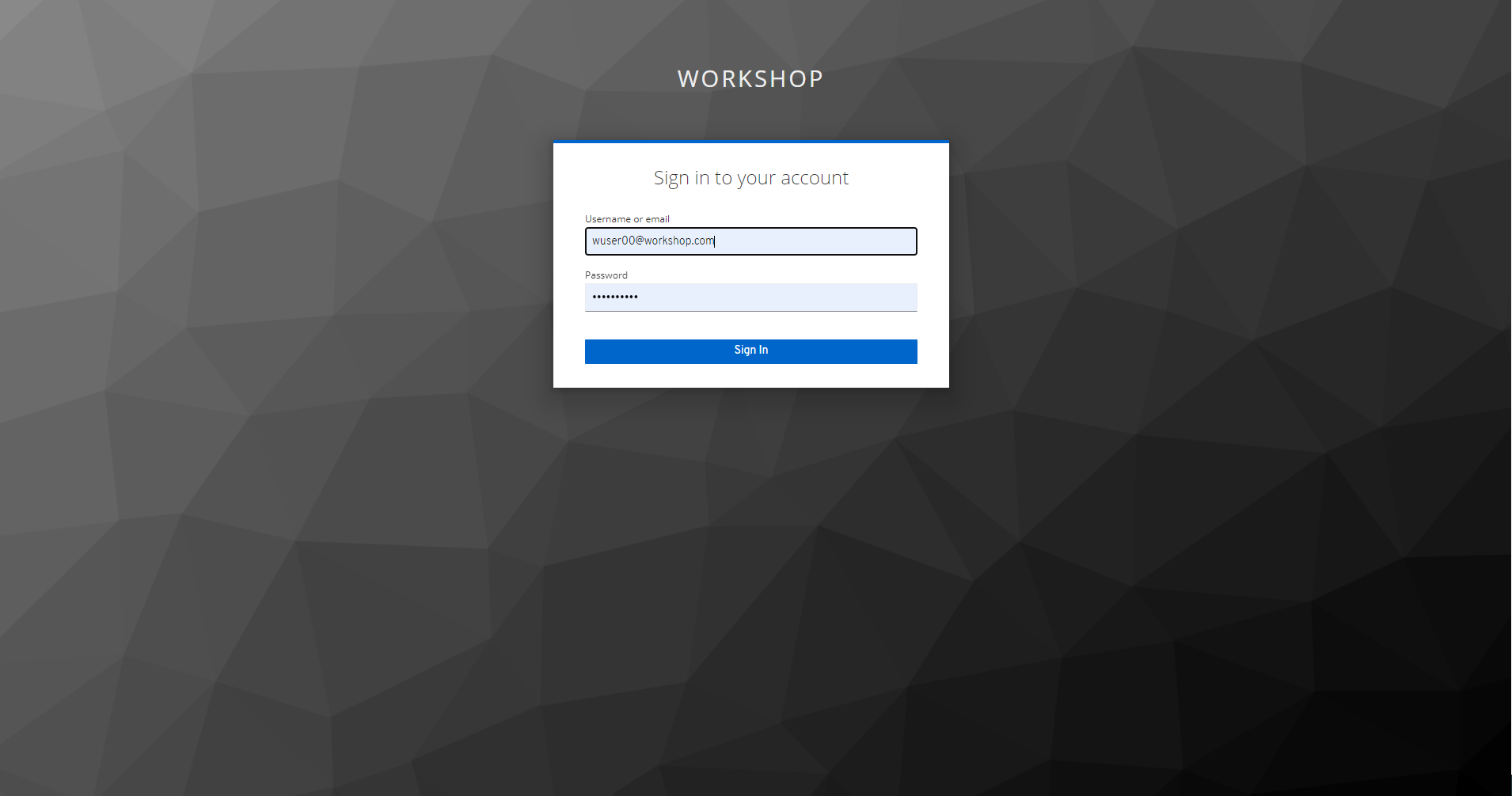
Please use the login URL: Workshop login.
Enter the Workshop Login Username and Workshop Login Password shared by your instructor.
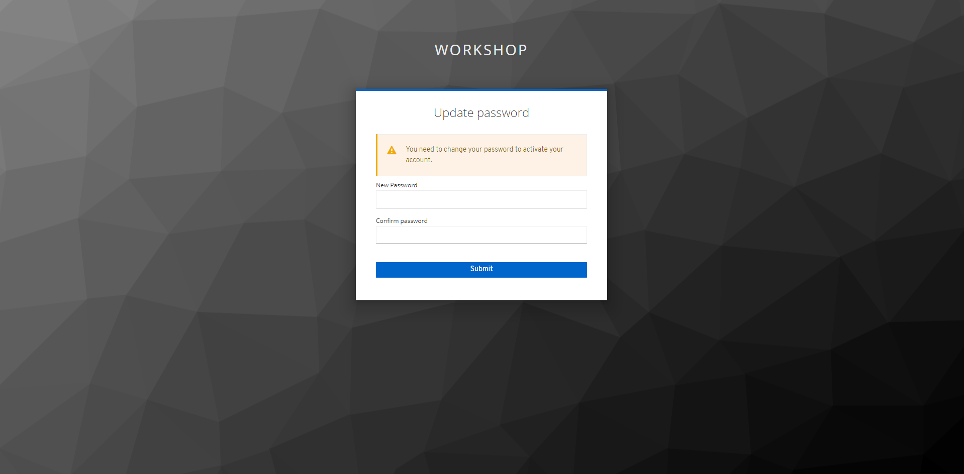
You will need to define your CDP Workload Password that will be used to acess non-SSO interfaces. You may read more about it here.
Please keep it with you. If you have forgotten it, you will be able to repeat this process and define another one.
-
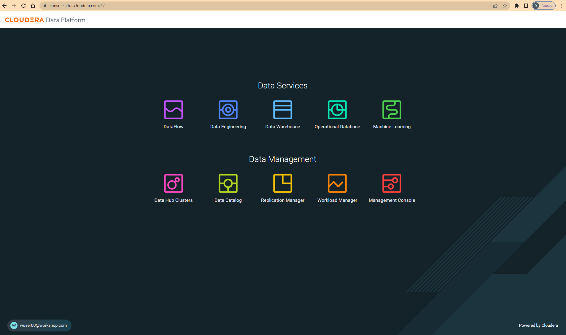
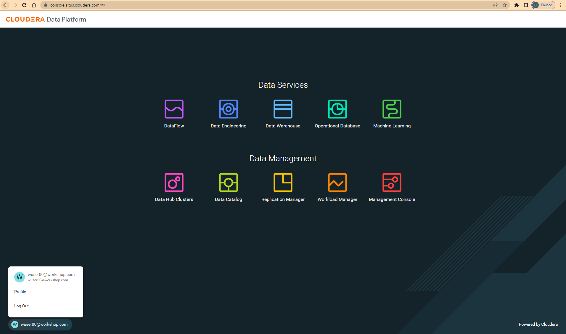
Click on your
user name (Ex: wuser00@workshop.com) at the lower left corner. -
Click on the
Profileoption.
-
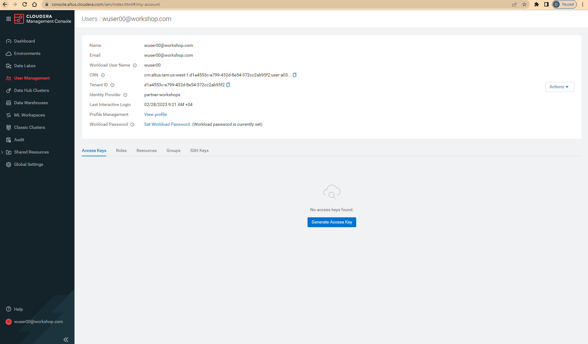
Click option
Set Workload Password. -
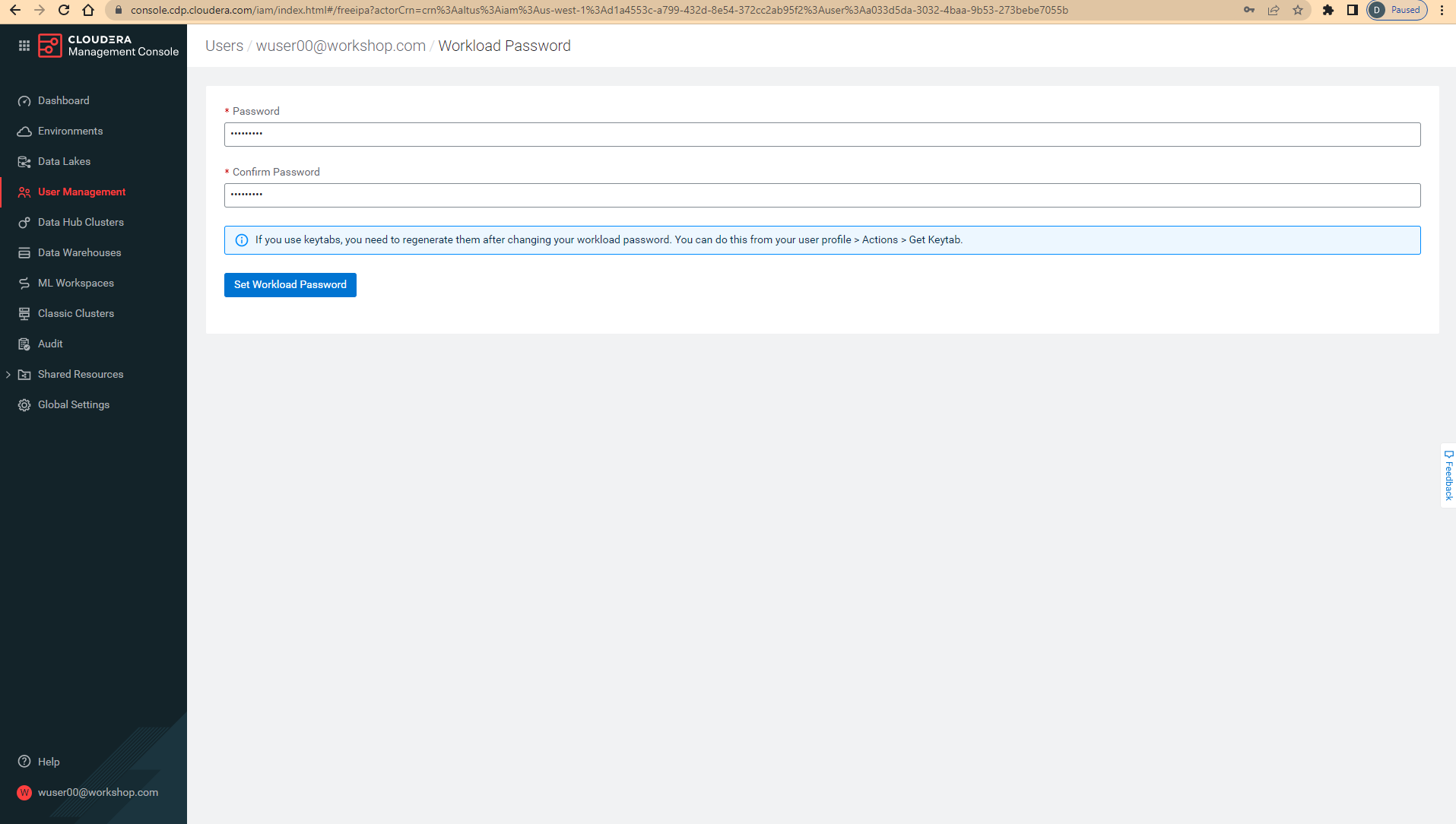
Enter a suitable
PasswordandConfirm Password. -
Click button
Set Workload Password.
Check that you got the message - Workload password is currently set or alternatively, look for a message next to Workload Password which says (Workload password is currently set)
In this step you’ll explore how to take advantage of CDW.
|
Warning
|
INSTRUCTOR WILL WALK YOU THROUGH THE ENVIRONMENT. |
Click the below for Virtual Tour Experience(s):
(a) CDW Virtual Tour
(b) Virtual Tour of CDP & Other Data Services
Click the below for Detailed Documentation(s):
(a) Getting Started in CDW
(b) CDP Public Cloud Data Warehouse
(c) CDP Private Cloud Getting Started
The objective of this step is to create External tables on top of raw CSV files sitting in cloud storage (In this case it has been stored in AWS S3 by the instructor) and then run few queries to access the data via SQL using HUE.
CREATE DATABASE ${user_id}_airlines_raw;

CREATE DATABASE ${user_id}_airlines;-
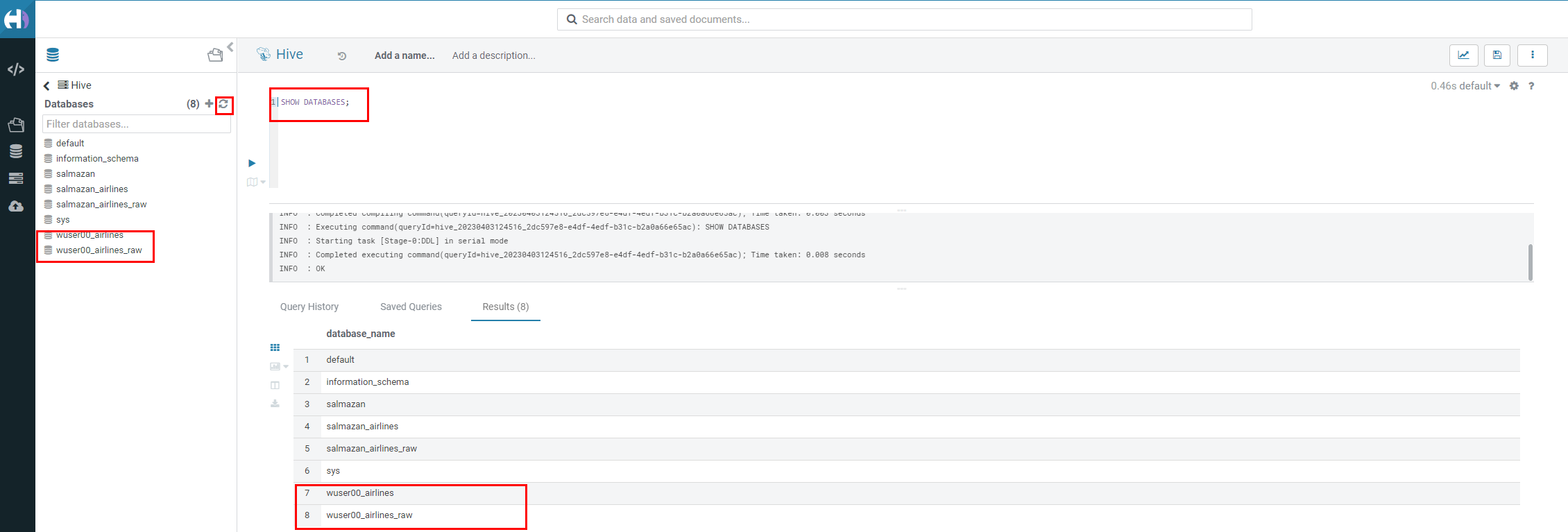
There may be many databases, look for the 2 that start with your
<user_id>. Run the following SQL to see the 2 databases that you created just now.
SHOW DATABASES;This will create External Tables on CSV Data Files that have been uploaded previously by your instructor in AWS S3. This provides a fast way to allow SQL layer on top of data in cloud storage.
-
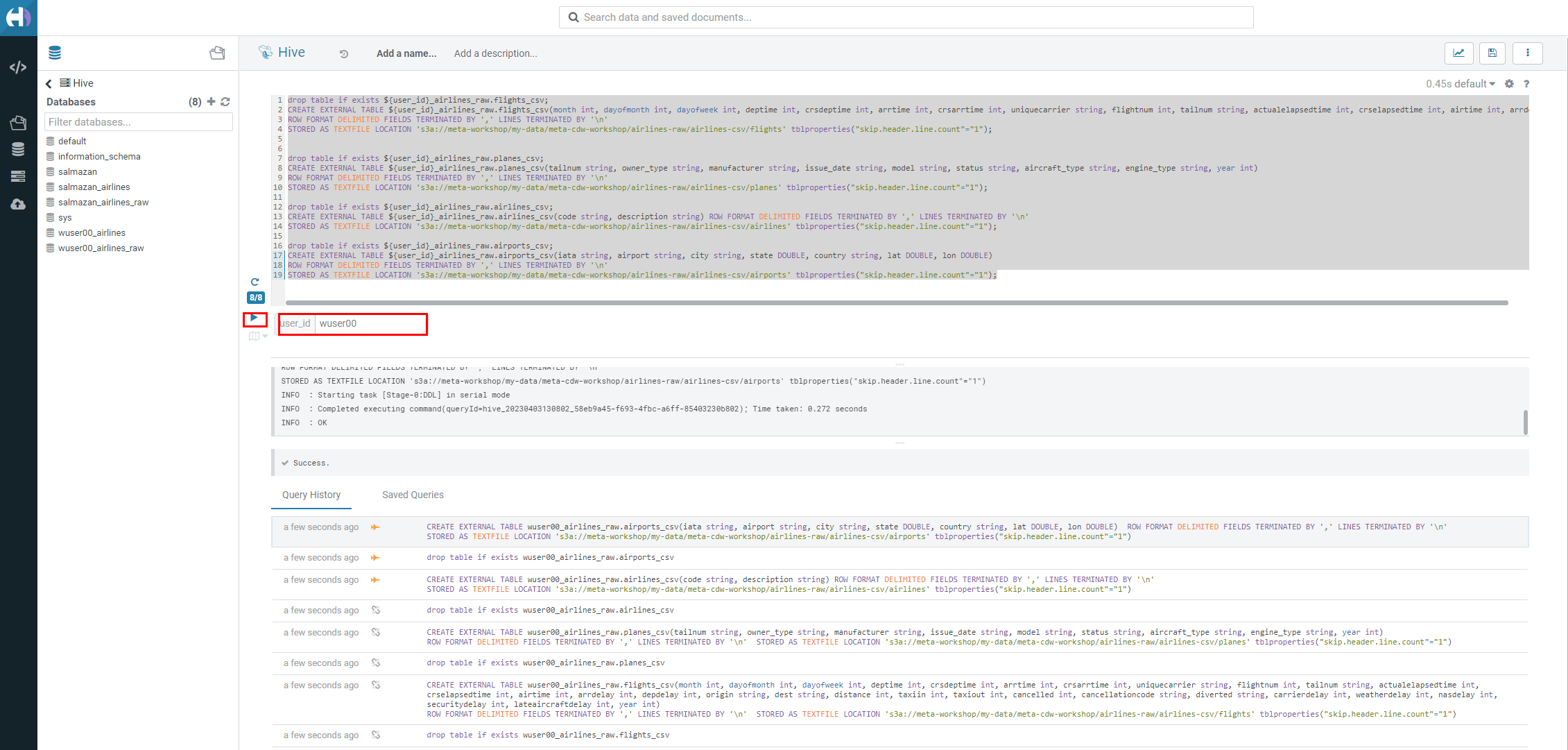
Copy paste the following into HUE.
drop table if exists ${user_id}_airlines_raw.flights_csv;
CREATE EXTERNAL TABLE ${user_id}_airlines_raw.flights_csv(month int, dayofmonth int, dayofweek int, deptime int, crsdeptime int, arrtime int, crsarrtime int, uniquecarrier string, flightnum int, tailnum string, actualelapsedtime int, crselapsedtime int, airtime int, arrdelay int, depdelay int, origin string, dest string, distance int, taxiin int, taxiout int, cancelled int, cancellationcode string, diverted string, carrierdelay int, weatherdelay int, nasdelay int, securitydelay int, lateaircraftdelay int, year int)
ROW FORMAT DELIMITED FIELDS TERMINATED BY ',' LINES TERMINATED BY '\n'
STORED AS TEXTFILE LOCATION 's3a://emeaworkshop/my-data/meta-cdw-workshop/airlines-raw/airlines-csv/flights' tblproperties("skip.header.line.count"="1");

drop table if exists ${user_id}_airlines_raw.planes_csv;
CREATE EXTERNAL TABLE ${user_id}_airlines_raw.planes_csv(tailnum string, owner_type string, manufacturer string, issue_date string, model string, status string, aircraft_type string, engine_type string, year int)
ROW FORMAT DELIMITED FIELDS TERMINATED BY ',' LINES TERMINATED BY '\n'
STORED AS TEXTFILE LOCATION 's3a://emeaworkshop/my-data/meta-cdw-workshop/airlines-raw/airlines-csv/planes' tblproperties("skip.header.line.count"="1");

drop table if exists ${user_id}_airlines_raw.airlines_csv;
CREATE EXTERNAL TABLE ${user_id}_airlines_raw.airlines_csv(code string, description string) ROW FORMAT DELIMITED FIELDS TERMINATED BY ',' LINES TERMINATED BY '\n'
STORED AS TEXTFILE LOCATION 's3a://emeaworkshop/my-data/meta-cdw-workshop/airlines-raw/airlines-csv/airlines' tblproperties("skip.header.line.count"="1");

drop table if exists ${user_id}_airlines_raw.airports_csv;
CREATE EXTERNAL TABLE ${user_id}_airlines_raw.airports_csv(iata string, airport string, city string, state DOUBLE, country string, lat DOUBLE, lon DOUBLE)
ROW FORMAT DELIMITED FIELDS TERMINATED BY ',' LINES TERMINATED BY '\n'
STORED AS TEXTFILE LOCATION 's3a://emeaworkshop/my-data/meta-cdw-workshop/airlines-raw/airlines-csv/airports' tblproperties("skip.header.line.count"="1");-
Check all the 4 tables were created.
USE ${user_id}_airlines_raw;

SHOW TABLES;
Make sure that 4 tables (airlines_csv, airports_csv, flights_csv, planes_csv) are created as shown below.
Now, copy paste the following in the HUE browser and click on Run as shown below.
select count(*) from ${user_id}_airlines_raw.flights_csv;Notice that while the query is executing, continue to the next step. Once the query returns you will see the following in the Results - the flights_csv table has over 86 million records.

Here, you’ll notice that the warehouse is now at a state where it is not executing any queries and hence, the node count would be low and as the users will run their queries it will scale up or down depending upon the need of resources or lack of it when queries are not run.
-
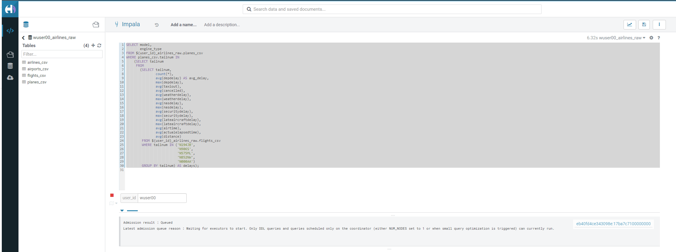
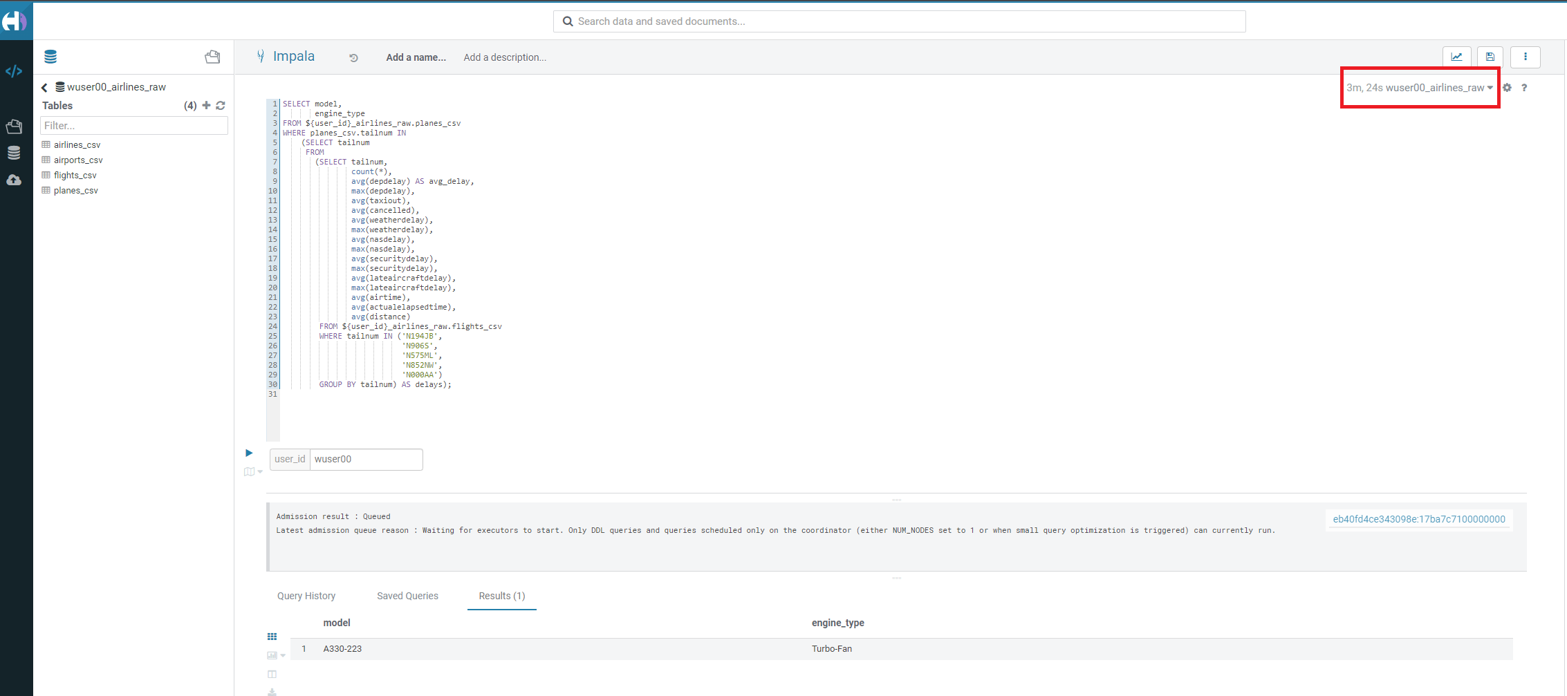
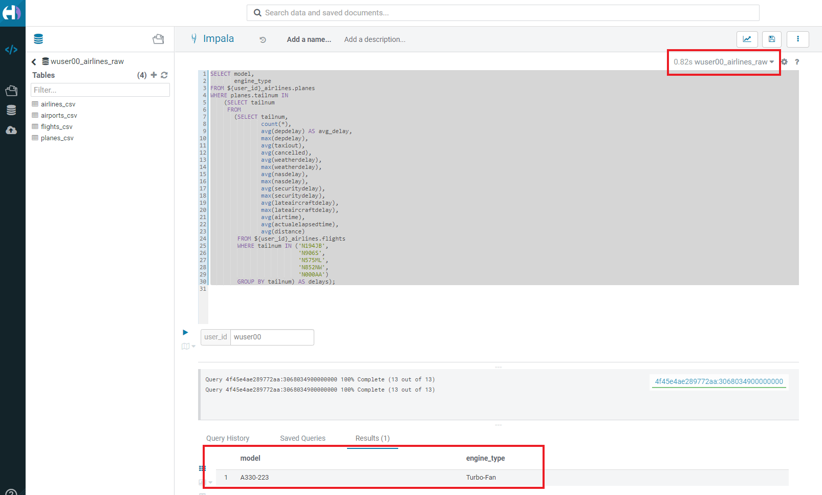
Run the following query to start analysing the data - “Find the needle in the haystack” query.
SELECT model,
       engine_type
FROM ${user_id}_airlines_raw.planes_csv
WHERE planes_csv.tailnum IN
    (SELECT tailnum
     FROM
       (SELECT tailnum,
               count(*),
               avg(depdelay) AS avg_delay,
               max(depdelay),
               avg(taxiout),
               avg(cancelled),
               avg(weatherdelay),
               max(weatherdelay),
               avg(nasdelay),
               max(nasdelay),
               avg(securitydelay),
               max(securitydelay),
               avg(lateaircraftdelay),
               max(lateaircraftdelay),
               avg(airtime),
               avg(actualelapsedtime),
               avg(distance)
        FROM ${user_id}_airlines_raw.flights_csv
        WHERE tailnum IN ('N194JB',
                          'N906S',
                          'N575ML',
                          'N852NW',
                          'N000AA')
GROUP BY tailnum) AS delays);In this step we will take steps to make use of Hive and Iceberg Table formats to provide us with best of both world scenarios in our Data Lakehouse. We will -
4.1 Create a curated layer from RAW CSV Tables (Created in Step 3). Curated layer will be created in <user_id>_airlines - This will be our 'Data Lakehouse'. Data Lakehouse will be combination of 2 Table Formats (Hive & Iceberg).
4.2 Migrate over time from Hive to Iceberg Table format and hence have the choice to not have to migrate everything at once.
4.2.1 Utilize the table Migration feature.
4.2.2 Use Create Table as Select (CTAS).
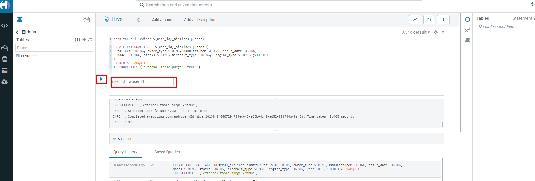
drop table if exists ${user_id}_airlines.planes;

CREATE EXTERNAL TABLE ${user_id}_airlines.planes (
  tailnum STRING, owner_type STRING, manufacturer STRING, issue_date STRING,
  model STRING, status STRING, aircraft_type STRING,  engine_type STRING, year INT
)
STORED AS PARQUET
TBLPROPERTIES ('external.table.purge'='true');-
Load
planestable with data from the Raw layer tableplanes_csv.
INSERT INTO ${user_id}_airlines.planes
SELECT * FROM ${user_id}_airlines_raw.planes_csv;-
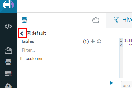
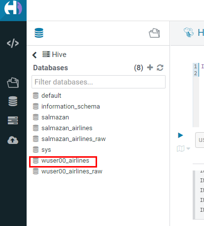
Switch to
<user_id>_airlinesdatabase by clicking the<option to the left ofdefaultdatabase. Click on<user_id>_airlinesdatabase. You should see theplanestable.
-
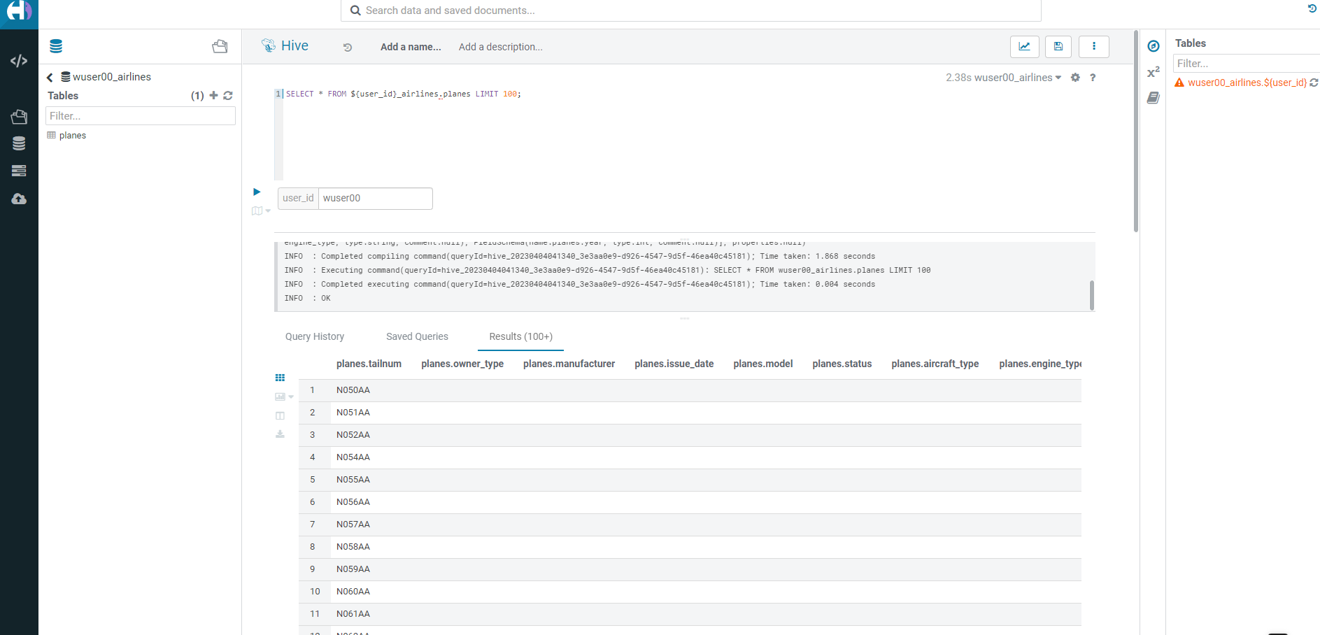
Run the SQL to see if the
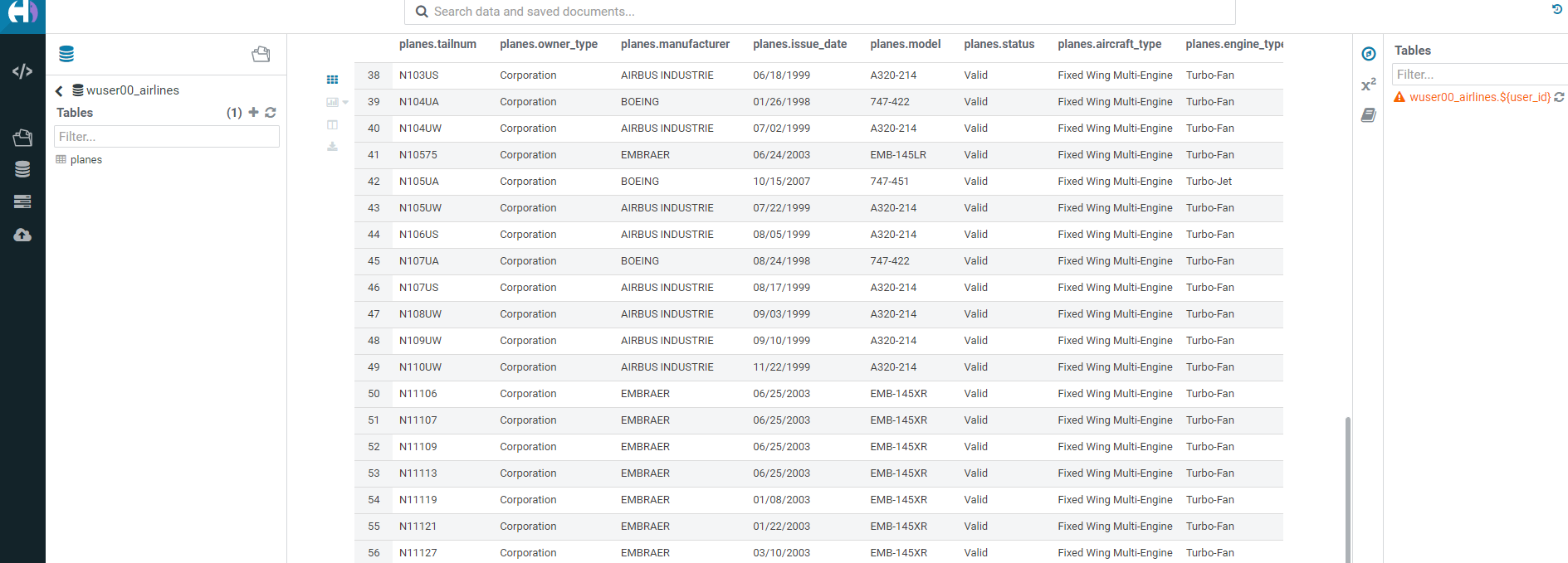
planestable was loaded correctly. Since,parquetuses highly efficient column-wise compression which occupies much disk space than CSV file and hence makes it faster to scan data in theparquetfile.
SELECT * FROM ${user_id}_airlines.planes LIMIT 100;Scroll down to see more values for the data.
-
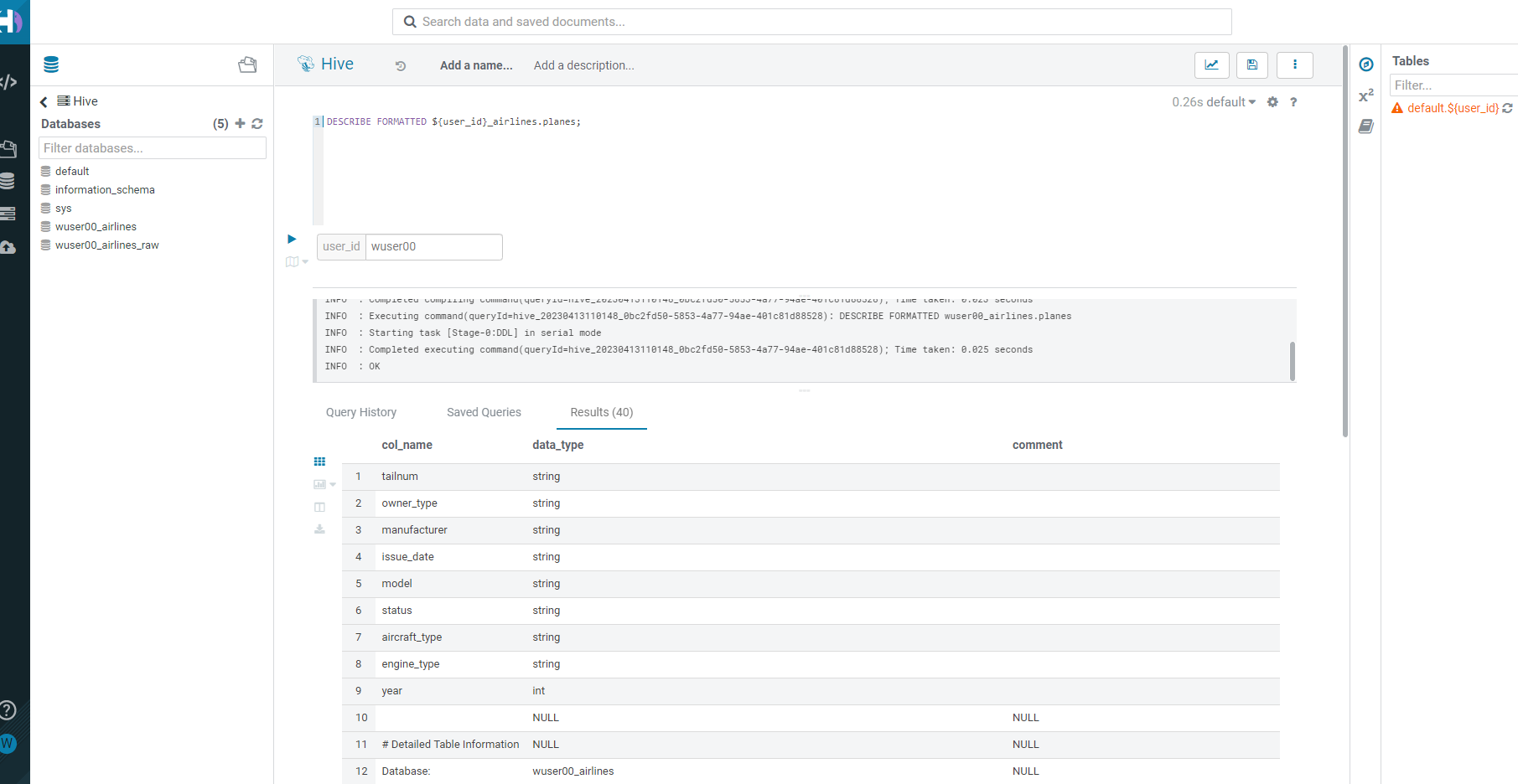
Execute the following command.
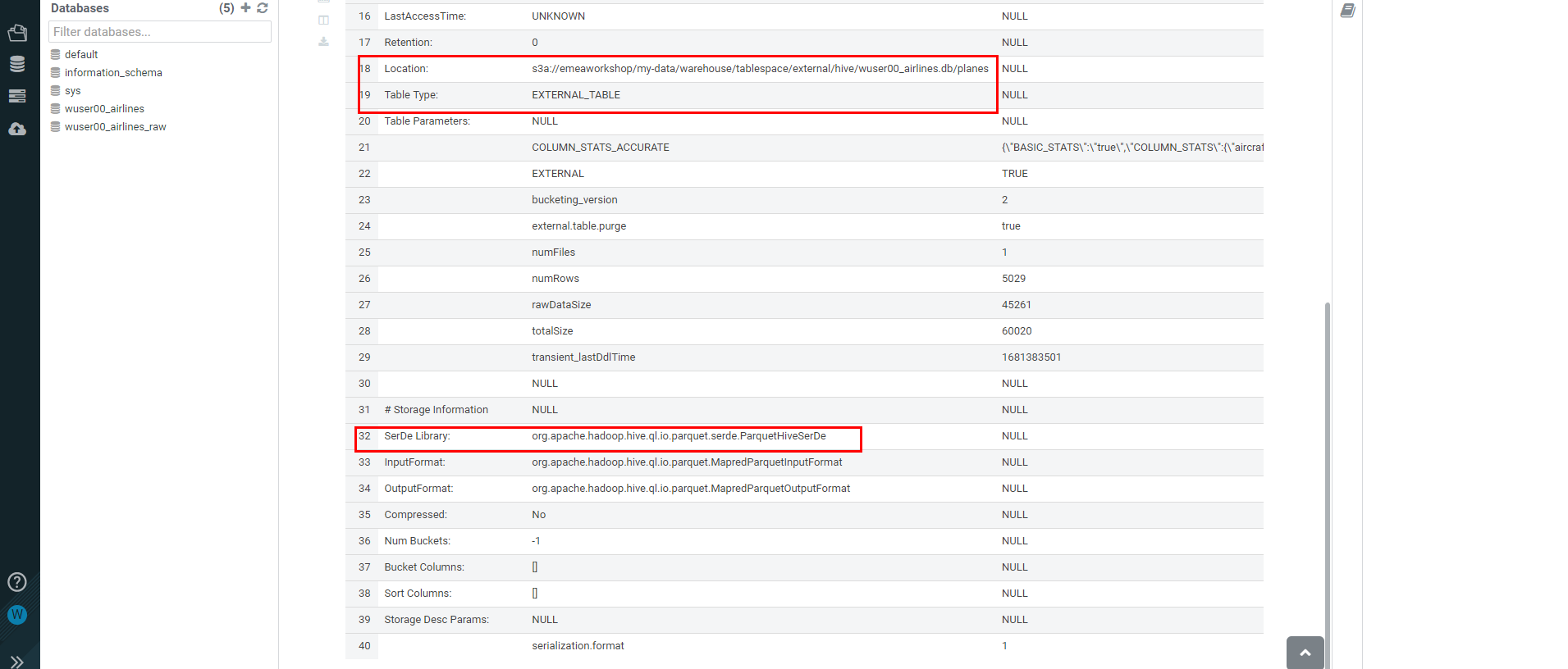
DESCRIBE FORMATTED ${user_id}_airlines.planes;In the output look for the following.
(a) Location: s3a://emeaworkshop/my-data/warehouse/tablespace/external/hive/wuser00_airlines.db/planes
(b) Table Type: EXTERNAL_TABLE
(c) SerDe Library: org.apache.hadoop.hive.ql.io.parquet.serde.ParquetHiveSerDe
-
Create
airlinestable inHivetable format andorcfile format. This table should also be fullyACIDcapable. We will useCreate Table As Select (CTAS). Since,airlinestable can change we need the ability toInsert/Update/Deleterecords.
drop table if exists ${user_id}_airlines.airlines_orc;
CREATE TABLE ${user_id}_airlines.airlines_orc
STORED AS ORC
AS
SELECT * FROM ${user_id}_airlines_raw.airlines_csv;-
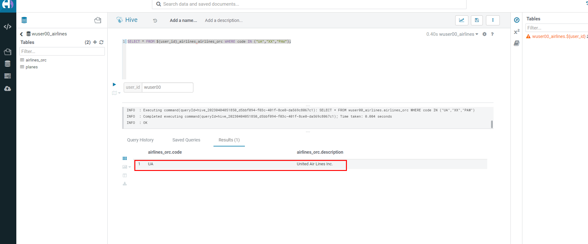
Run the following query to check data in the
airlines_orctable and it should return only 1 row for code 'UA'.
SELECT * FROM ${user_id}_airlines.airlines_orc WHERE code IN ("UA","XX","PAW");-
We shall now add a new record to the
airlines_orctable to see some Hive ACID capabilities.
INSERT INTO ${user_id}_airlines.airlines_orc VALUES("PAW","Paradise Air");-
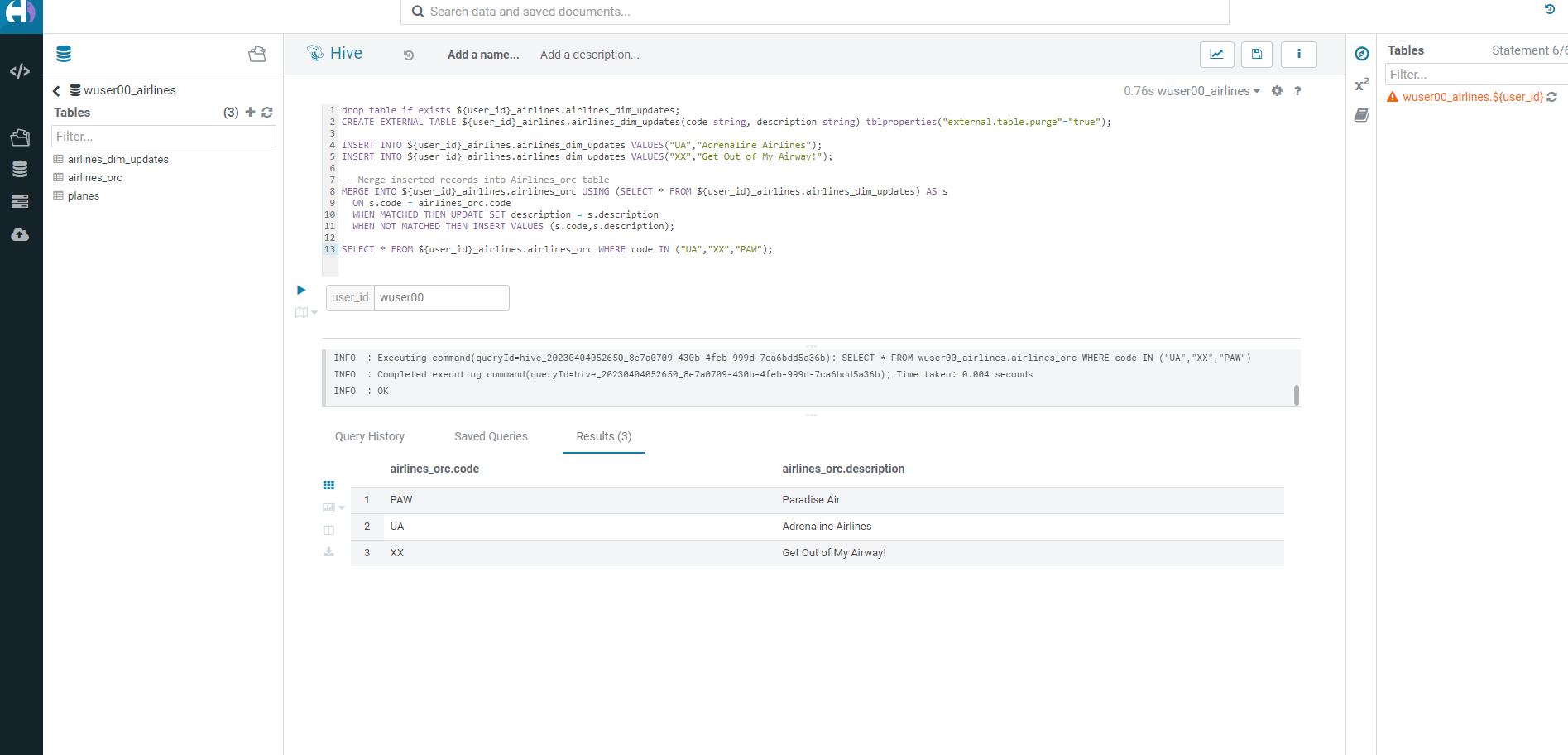
Let’s update an existing record to change the description of
United AirlinestoAdrenaline Airlinesto see more of theACIDcapablities provided by Hive ACID. Run the following SQL.
drop table if exists ${user_id}_airlines.airlines_dim_updates;
CREATE EXTERNAL TABLE ${user_id}_airlines.airlines_dim_updates(code string, description string) tblproperties("external.table.purge"="true");

INSERT INTO ${user_id}_airlines.airlines_dim_updates VALUES("UA","Adrenaline Airlines");
INSERT INTO ${user_id}_airlines.airlines_dim_updates VALUES("XX","Get Out of My Airway!");

-- Merge inserted records into Airlines_orc table
MERGE INTO ${user_id}_airlines.airlines_orc USING (SELECT * FROM ${user_id}_airlines.airlines_dim_updates) AS s
  ON s.code = airlines_orc.code
  WHEN MATCHED THEN UPDATE SET description = s.description
  WHEN NOT MATCHED THEN INSERT VALUES (s.code,s.description);

SELECT * FROM ${user_id}_airlines.airlines_orc WHERE code IN ("UA","XX","PAW");If you already have created a Data Warehouse using the Hive Table Format but would like to take advantage of the features offered in the Iceberg Table Format, you have 2 options. We will see both the options as a part of this step.
-
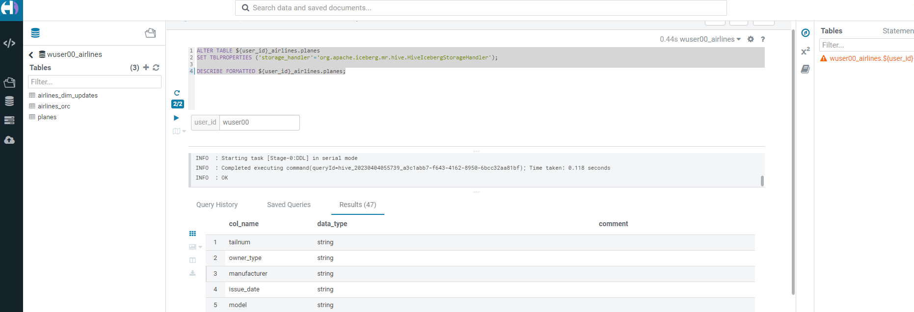
Run the following SQL and note what happens next.
ALTER TABLE ${user_id}_airlines.planes
SET TBLPROPERTIES ('storage_handler'='org.apache.iceberg.mr.hive.HiveIcebergStorageHandler');

DESCRIBE FORMATTED ${user_id}_airlines.planes;
The following happened.
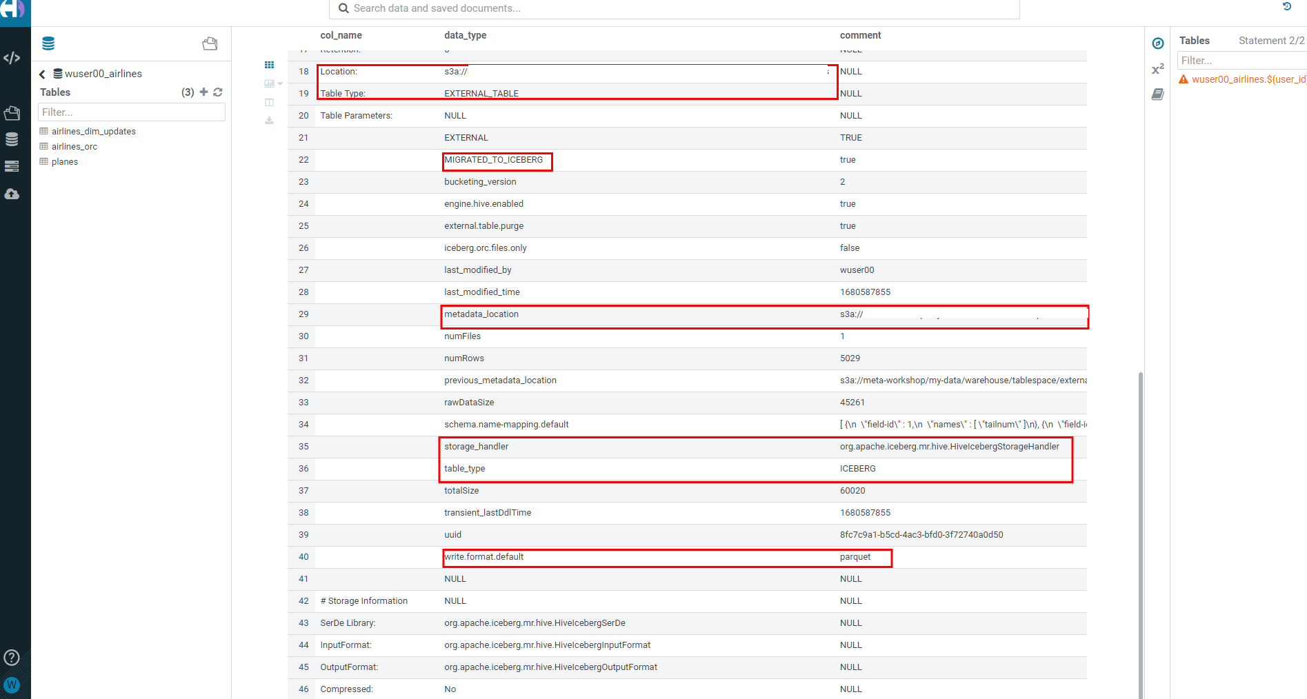
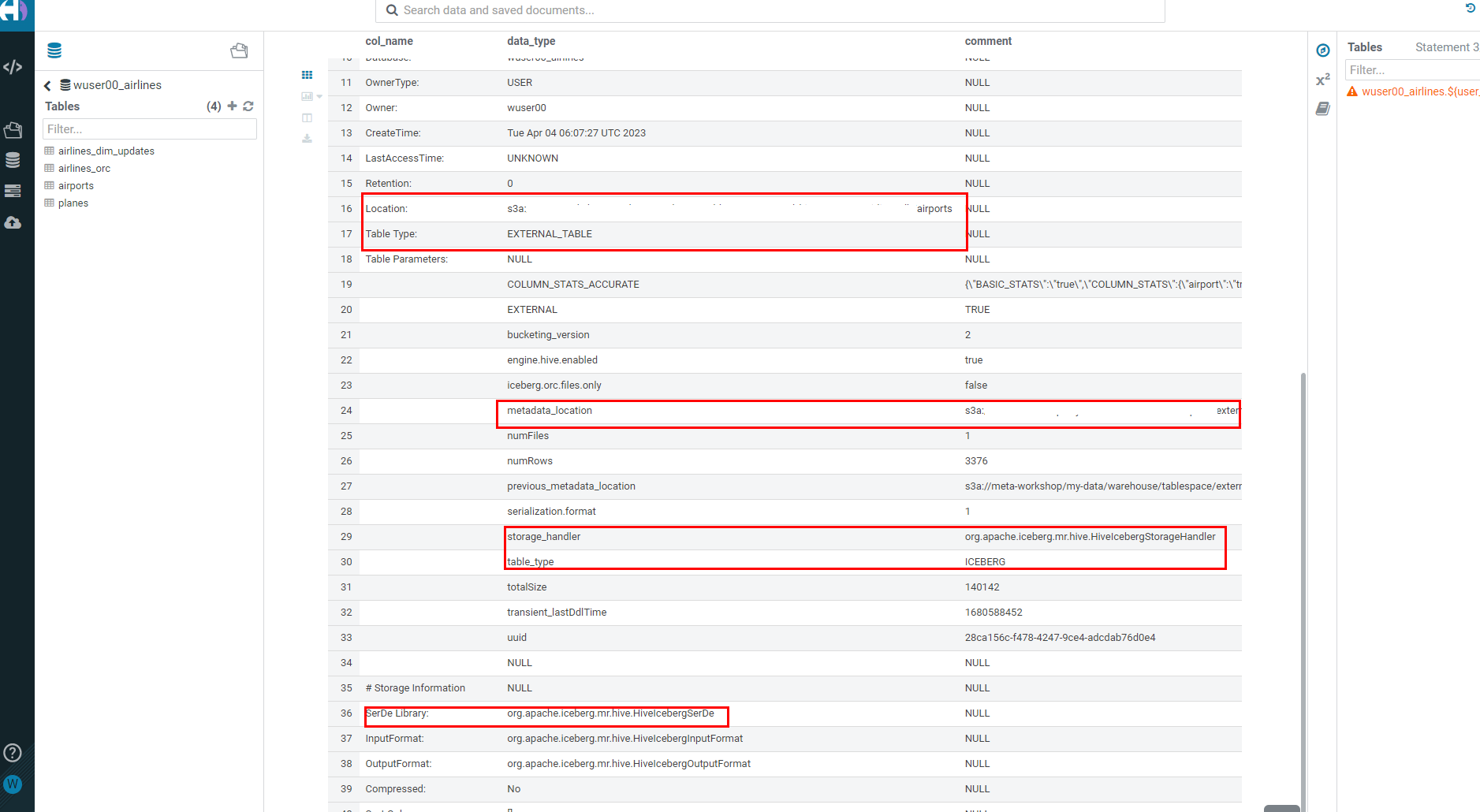
(a). This migration to Iceberg happened in-place & there was no re-writing of data that occurred as part of this process. It retained the File Format of parquet for the Iceberg table as well. There was a Metadata file that is created, which you can see when you run the DESCRIBE FORMATTED.
(b). In the output look for the following fields - look for the following (see image with highlighted fields) key values:
Table Type, Location (location of where table data is stored), SerDe Library, and in Table Parameters look for properties MIGRATED_TO_ICEBERG, storage_handler, metadata_location, and table_type.
Location - Data is stored in cloud storage and in this case AWS S3 in the same location as the Hive Table Format.
Table Type: Indicates that it is an EXTERNAL TABLE.
MIGRATED_TO_ICEBERG: Indicates that the table has migrated to ICEBERG.
table_type: Indicates ICEBERG table format.
metadata_location: Indicates the location of metadata which is path to cloud storage.
storage_handler: org.apache.iceberg.mr.hive.HiveIcebergStorageHandler.
SerDe Library: org.apache.iceberg.mr.hive.HiveIcebergSerDe.
-
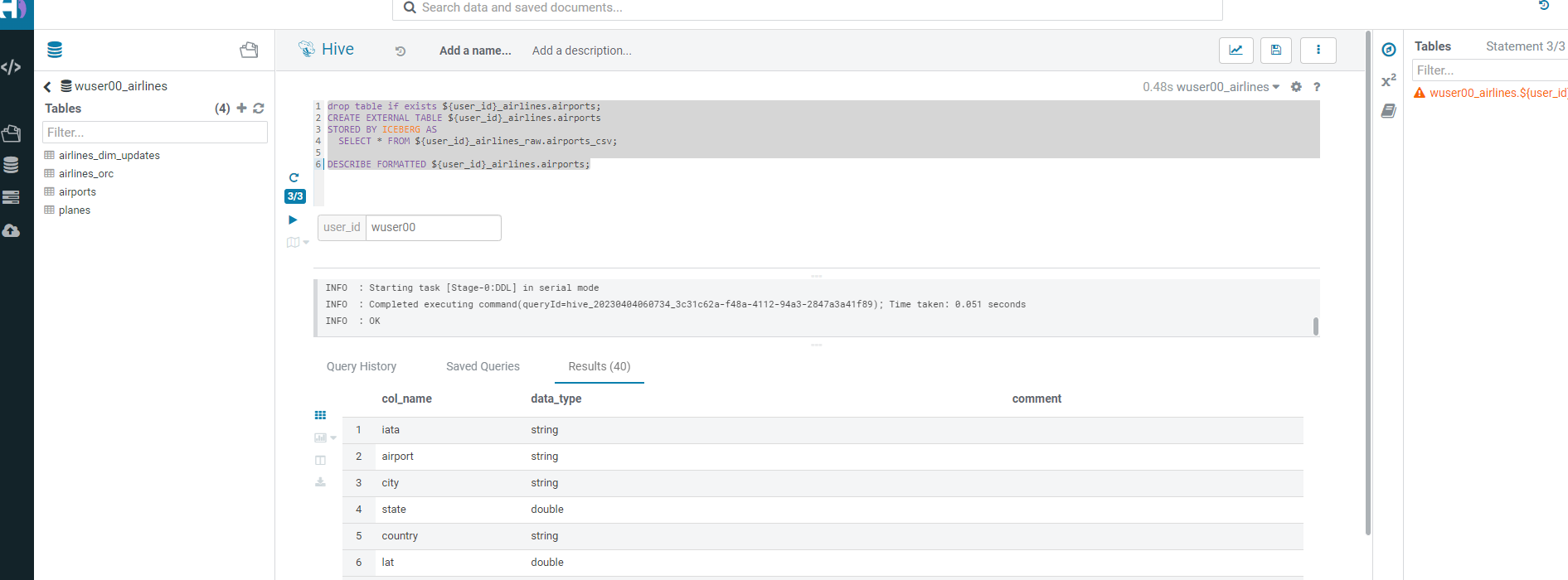
Run the following SQL to create
airportstable using CTAS. Notice the syntax to create an Iceberg Table within Hive isStored by Iceberg.
drop table if exists ${user_id}_airlines.airports;
CREATE EXTERNAL TABLE ${user_id}_airlines.airports
STORED BY ICEBERG AS
  SELECT * FROM ${user_id}_airlines_raw.airports_csv;

DESCRIBE FORMATTED ${user_id}_airlines.airports;
Look for: Table Type, Location (location of where table data is stored), SerDe Library, and in Table Parameters look for properties storage_handler, metadata_location, and table_type.
-
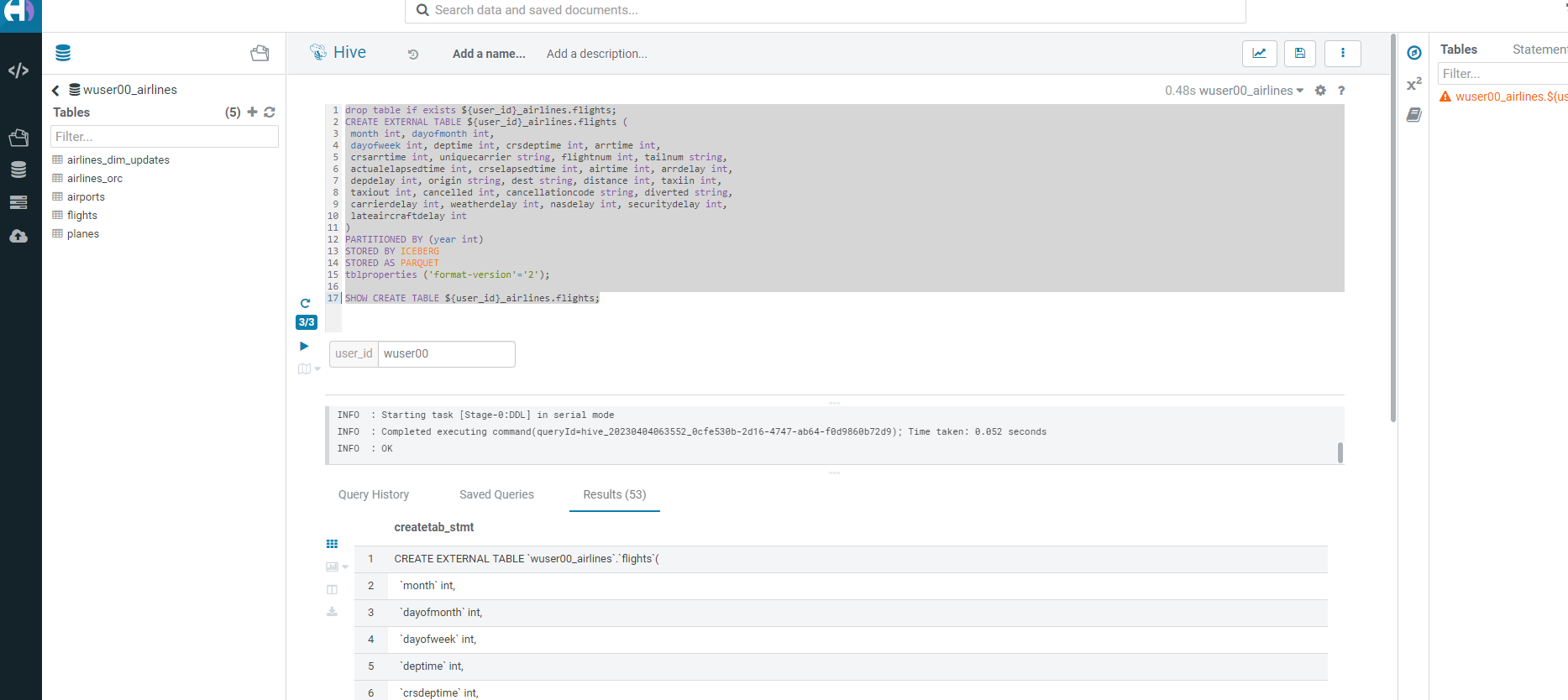
In this step we will create a partitioned table, in
IcebergTable Format, stored inParquetFile Format. Other than that we could specify other file formats that are supported for Iceberg which are:ORC and Avro.
drop table if exists ${user_id}_airlines.flights;
CREATE EXTERNAL TABLE ${user_id}_airlines.flights (
 month int, dayofmonth int,
 dayofweek int, deptime int, crsdeptime int, arrtime int,
 crsarrtime int, uniquecarrier string, flightnum int, tailnum string,
 actualelapsedtime int, crselapsedtime int, airtime int, arrdelay int,
 depdelay int, origin string, dest string, distance int, taxiin int,
 taxiout int, cancelled int, cancellationcode string, diverted string,
 carrierdelay int, weatherdelay int, nasdelay int, securitydelay int,
 lateaircraftdelay int
)
PARTITIONED BY (year int)
STORED BY ICEBERG
STORED AS PARQUET
tblproperties ('format-version'='2');

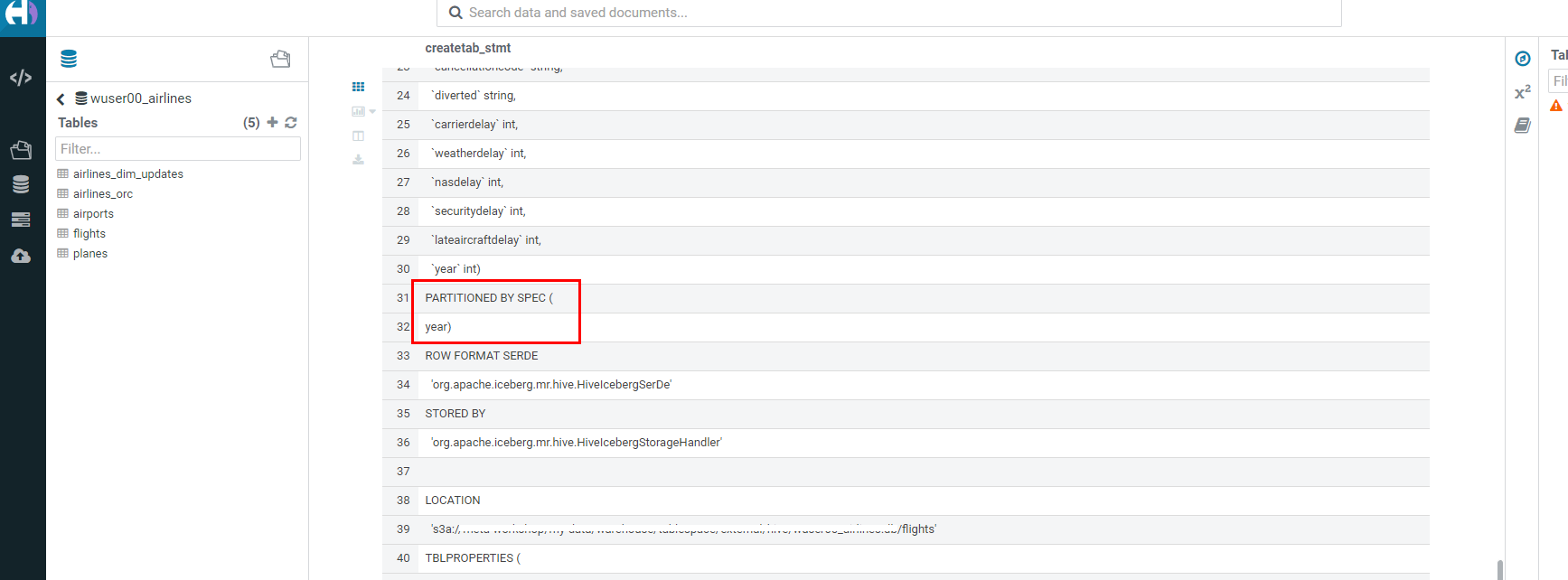
SHOW CREATE TABLE ${user_id}_airlines.flights;
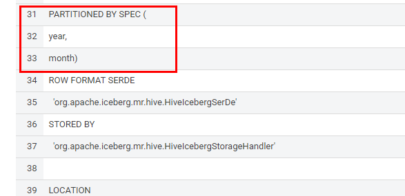
The SHOW CREATE TABLE command is the unformatted version of DESCRIBE FORMATTED command. Pay attention to the PARTITIONED BY SPEC, where we have partitioned the flights table using year column.
-
We insert data into this table it will write data together within the same partition (ie. all 2006 data is written to the same location, all 2005 data is written to the same location, etc.).
This command will take some time to run.
INSERT INTO ${user_id}_airlines.flights
SELECT * FROM ${user_id}_airlines_raw.flights_csv
WHERE year <= 2006;-
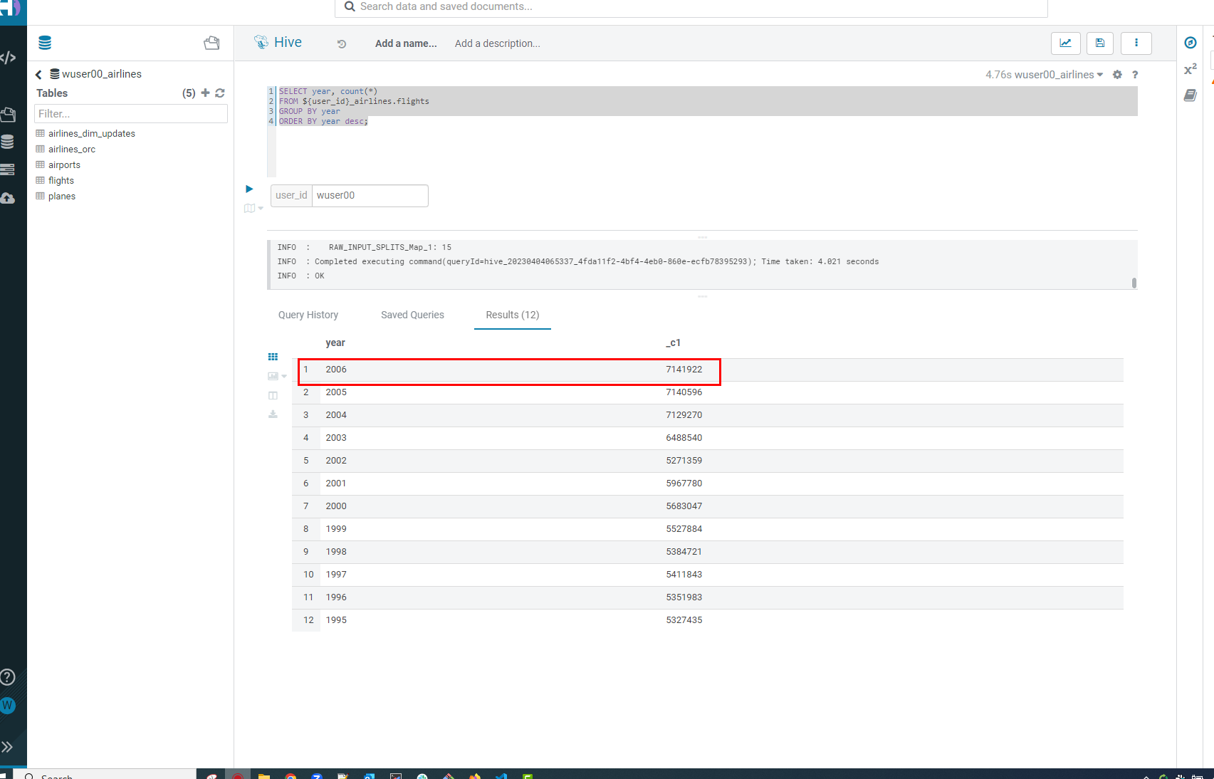
Run the following SQL and notice that each of the years have a range of data within a few million flights (each record in the flights table counts as a flight).
SELECT year, count(*)
FROM ${user_id}_airlines.flights
GROUP BY year
ORDER BY year desc;-
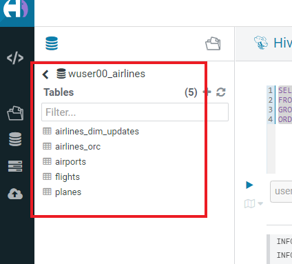
Now, make sure that the following 5 tables are created up until this point as shown in the screenshot below.
Below is the summary of what we have done so far in the form of a screenshot.
(1). Created a Raw Layer by defining Tables that point to CSV data files in an S3 bucket. We were then immediately able to query and run analytics against that data.
(2). Created a Curated Layer to be the basis of our Data Lakehouse.
-
(2.1). Created the
planestable in Hive table format stored inParquetto improve performance of querying this from the Raw CSV data due to how the data is stored. Migrated,in-place- no data rewrite, the planes table from Hive table format to Iceberg table format using the Migration utility (Alter Table statement). -
(2.2). Created the
airlines_orctable in Hive table format stored inORCto improve performance of querying this from the Raw CSV data due to how the data is stored. Took advantage of the HiveACIDcapabilities to Insert, Update, Delete, and Merge data into this table. Here we created a staging table to write new incoming data to be used to update theairlines_orctable with (Merge command). -
(2.3). Created the
airportstable in Iceberg Table Format using aCTASstatement querying the Raw CSV data to take advantage of the features of Iceberg. -
(2.4). Created the flights table in Iceberg Table Format and partitioned the table by the year column. Inserted data into the table up to year 2006.
As a final step here let’s run the same analytic query we ran against the Raw layer now in our Data Lakehouse DW, to see what happens with performance.
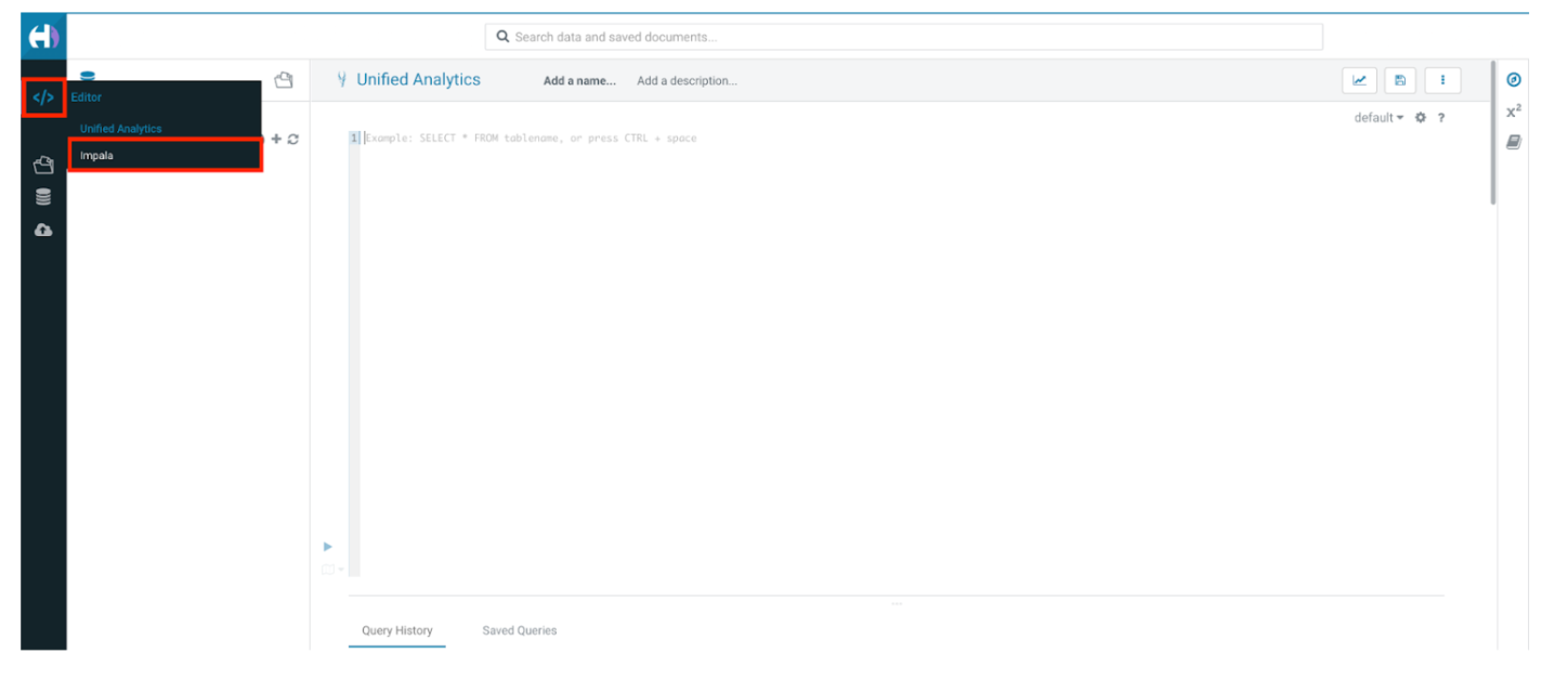
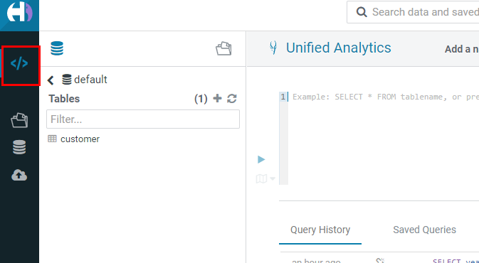
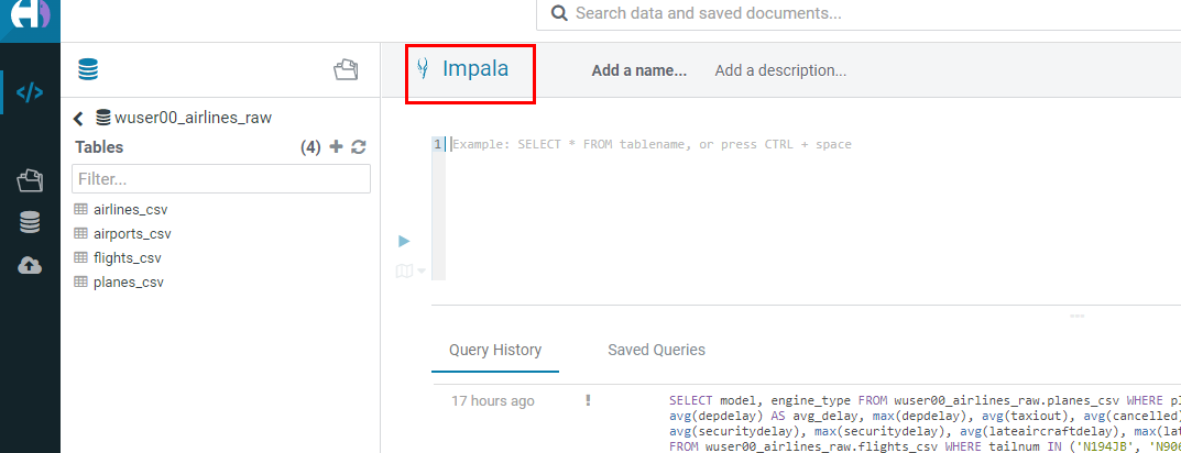
From the cloudera console click on - 1-10impala.
SELECT model,
       engine_type
FROM ${user_id}_airlines.planes
WHERE planes.tailnum IN
    (SELECT tailnum
     FROM
       (SELECT tailnum,
               count(*),
               avg(depdelay) AS avg_delay,
               max(depdelay),
               avg(taxiout),
               avg(cancelled),
               avg(weatherdelay),
               max(weatherdelay),
               avg(nasdelay),
               max(nasdelay),
               avg(securitydelay),
               max(securitydelay),
               avg(lateaircraftdelay),
               max(lateaircraftdelay),
               avg(airtime),
               avg(actualelapsedtime),
               avg(distance)
        FROM ${user_id}_airlines.flights
        WHERE tailnum IN ('N194JB',
                          'N906S',
                          'N575ML',
                          'N852NW',
                          'N000AA')
GROUP BY tailnum) AS delays);In this Step we will look at some of the performance optimization and table maintenance tasks that can be performed to ensure the best possible TCO, while ensuring the best performance.
ALTER TABLE ${user_id}_airlines.flights
SET PARTITION spec ( year, month );

SHOW CREATE TABLE ${user_id}_airlines.flights;INSERT INTO ${user_id}_airlines.flights
SELECT * FROM ${user_id}_airlines_raw.flights_csv
WHERE year = 2007;SELECT year, month, count(*)
FROM ${user_id}_airlines.flights
WHERE year = 2006 AND month = 12
GROUP BY year, month
ORDER BY year desc, month asc;-
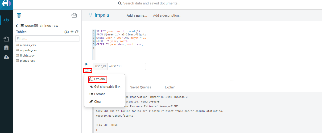
Copy/paste the following in the HUE Editor, but
DO NOTexecute the query.
SELECT year, month, count(*)
FROM ${user_id}_airlines.flights
WHERE year = 2007 AND month = 12
GROUP BY year, month
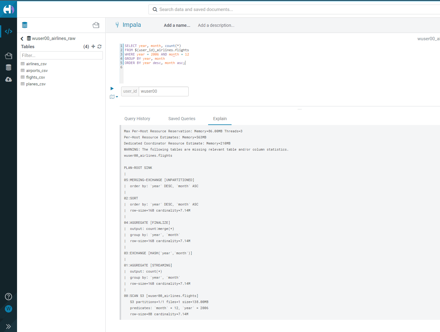
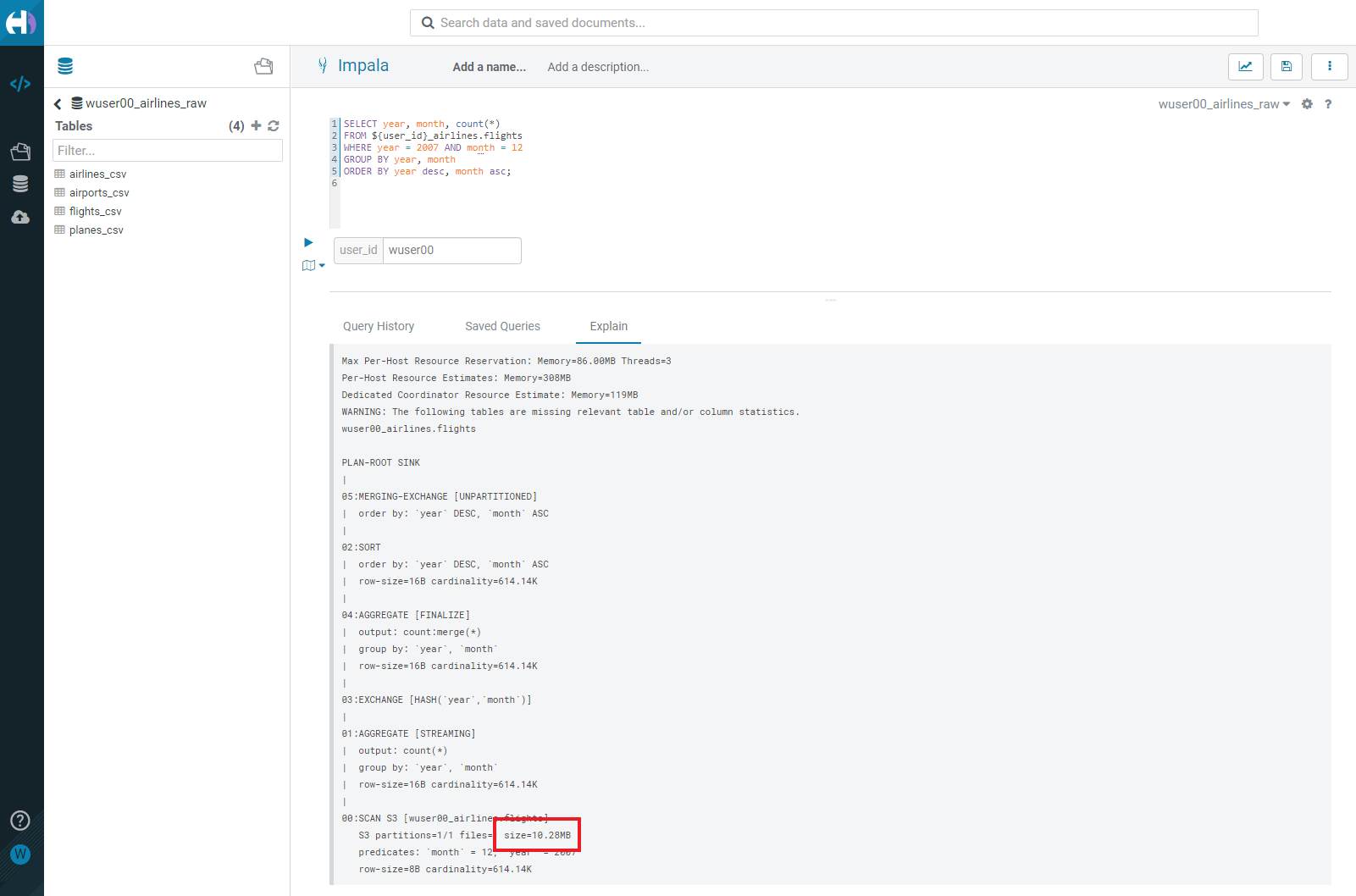
ORDER BY year desc, month asc;In the output notice the amount of data that needs to be scanned for this query, about 11 MB, is significantly less than that of the first, 138 MB. This shows an important capability of Iceberg, Partition Pruning. Meaning that much less data is scanned for this query and only the selected month of data needs to be processed. This should result in much faster query execution times.
-
In the previous steps we have loaded data into the
flightsiceberg table. We will insert more data into it. Each time we add (update or delete) data asnapshotis captured. The snapshot is important foreventual consistency& to allow multiple read/writes concurrently (from various engines or same engine).
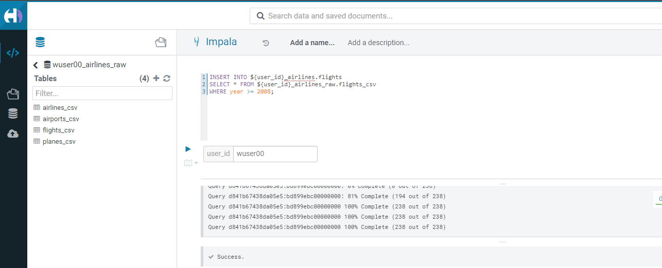
INSERT INTO ${user_id}_airlines.flights
SELECT * FROM ${user_id}_airlines_raw.flights_csv
WHERE year >= 2008;-
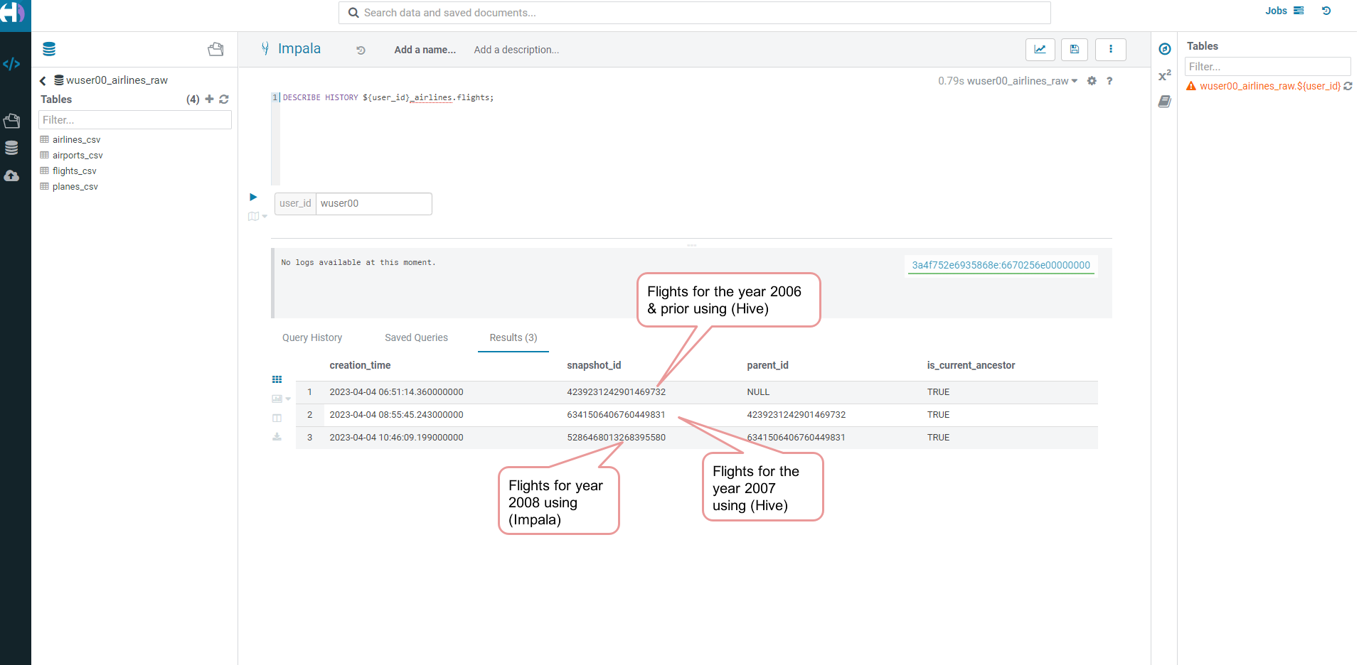
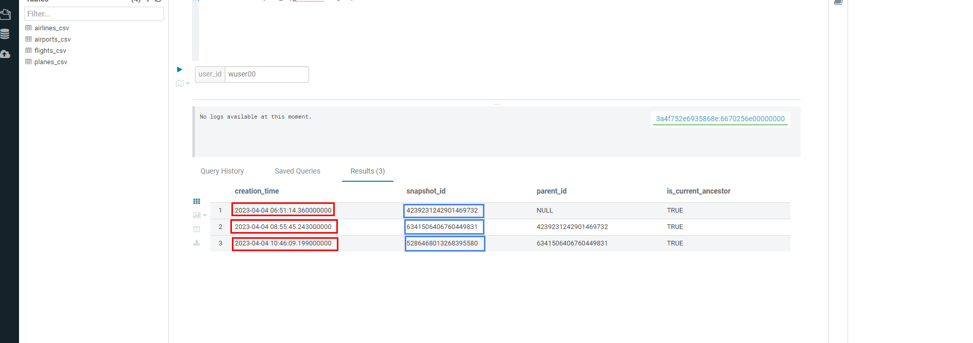
To see snapshots, execute the following SQL.
DESCRIBE HISTORY ${user_id}_airlines.flights;In the output there should be 3 Snapshots, described below. Note that we have been reading/writing data from/to the Iceberg table from both Hive & Impala. It is an important aspect of Iceberg Tables that they support multi-function analytics - ie. many engines can work with Iceberg tables (Cloudera Data Warehouse [Hive & Impala], Cloudera Data Engineering [Spark], Cloudera Machine Learning [Spark], Cloudera DataFlow [NiFi], and DataHub Clusters).
-
Copy/paste the following data into the Impala Editor, but
DO NOTexecute.
-- SELECT DATA USING TIMESTAMP FOR SNAPSHOT
SELECT year, count(*)
FROM ${user_id}_airlines.flights
  FOR SYSTEM_TIME AS OF '${create_ts}'
GROUP BY year
ORDER BY year desc;

-- SELECT DATA USING TIMESTAMP FOR SNAPSHOT
SELECT year, count(*)
FROM ${user_id}_airlines.flights
  FOR SYSTEM_VERSION AS OF ${snapshot_id}
GROUP BY year
ORDER BY year desc;-
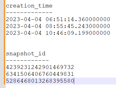
From the notepad just copy the first value of the timestamp. It could be the date or the timestamp. Paste it in the
create_tsbox. In our case the value was2023-04-04 06:51:14.360000000. Then execute the higlighted query only (1st query).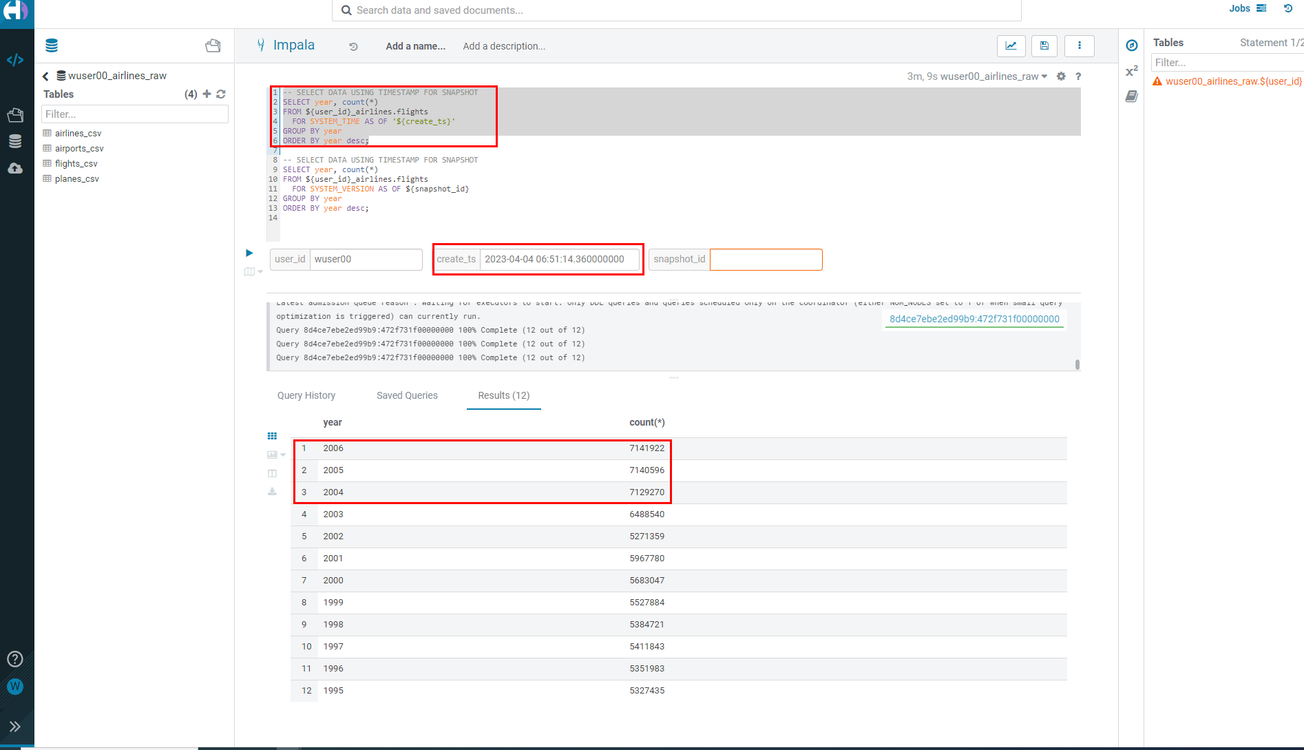
-
From the notepad just copy the second value of the snapshot id. In our case the value was
6341506406760449831. Paste it in thesnapshot_idbox. Then execute the higlighted query only (2nd query).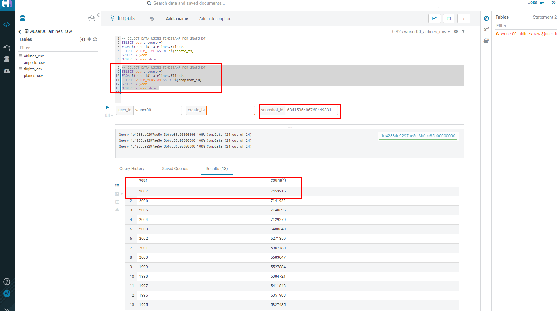
-
Sometimes data can be loaded incorrectly, due to many common issues - missing fields, only part of the data was loaded, bad data, etc. In situations like this data would need to be removed, corrected, and reloaded. Iceberg can help with the Rollback command to remove the “unwanted” data. This leverages Snapshot IDs to perform this action by using a simple ALTER TABLE command as follows. We will
NOT RUNthis command in this lab.
-- ALTER TABLE ${user_id}_airlines.flights EXECUTE ROLLBACK(${snapshot_id});-
As time passes it might make sense to expire old Snapshots, instead of the Snapshot ID you use the Timestamp to expire old Snapshots. You can do this manually by running a simple ALTER TABLE command as follows. We will
NOT RUNthis command in this lab.
-- Expire Snapshots up to the specified timestamp
-- BE CAREFUL: Once you run this you will not be able to Time Travel for any Snapshots that you Expire ALTER TABLE ${user_id}_airlines.flights
-- ALTER TABLE ${user_id}_airlines_maint.flights EXECUTE expire_snapshots('${create_ts}');-
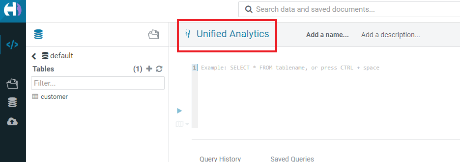
This can be used for both Iceberg tables and Hive Tables to improve performance. Go to the Cloudera console and look for
1-10hive. Click on theHuebutton on the right upper corner of1-10hiveas shown in the screenshot below.
-
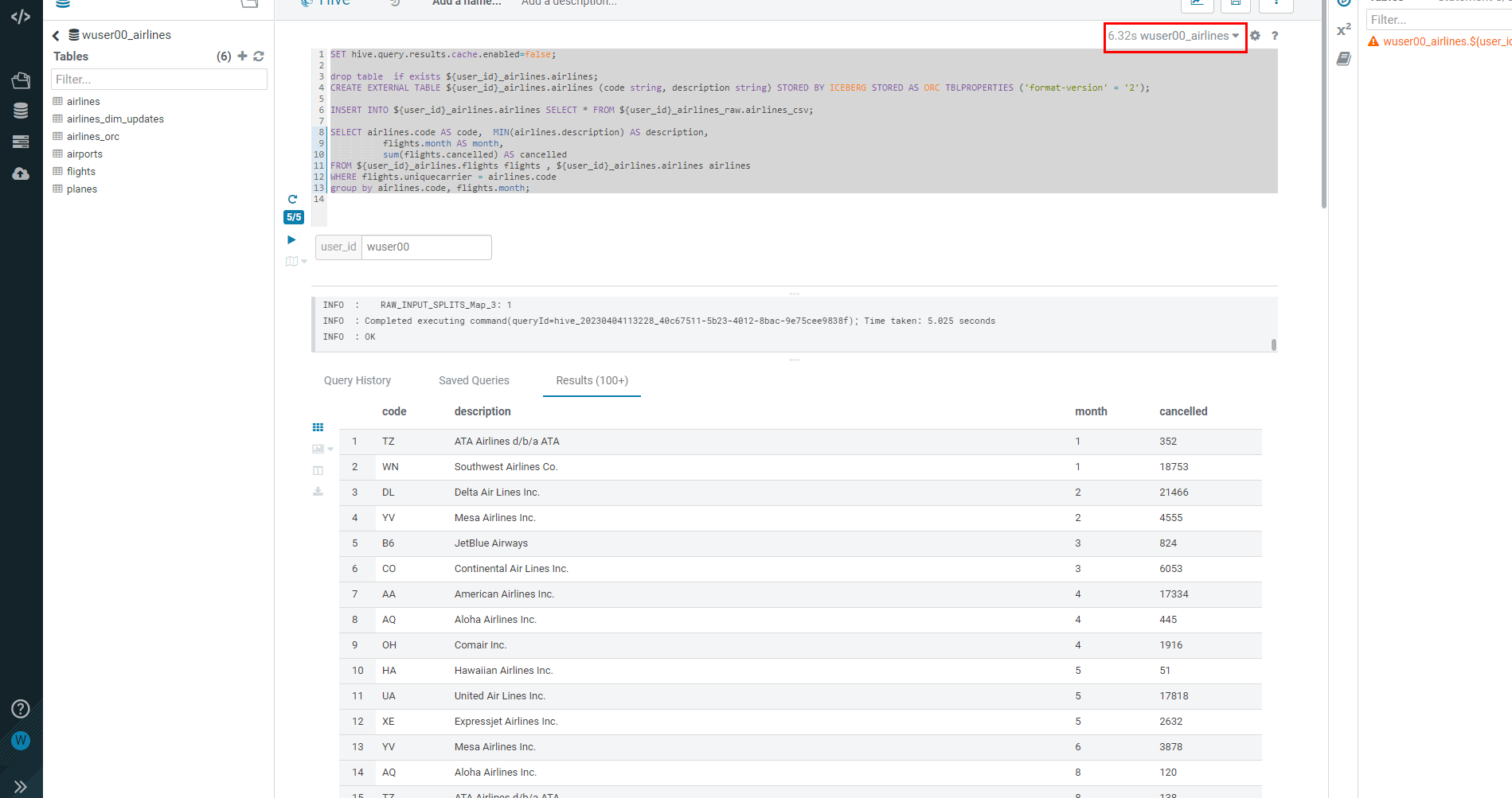
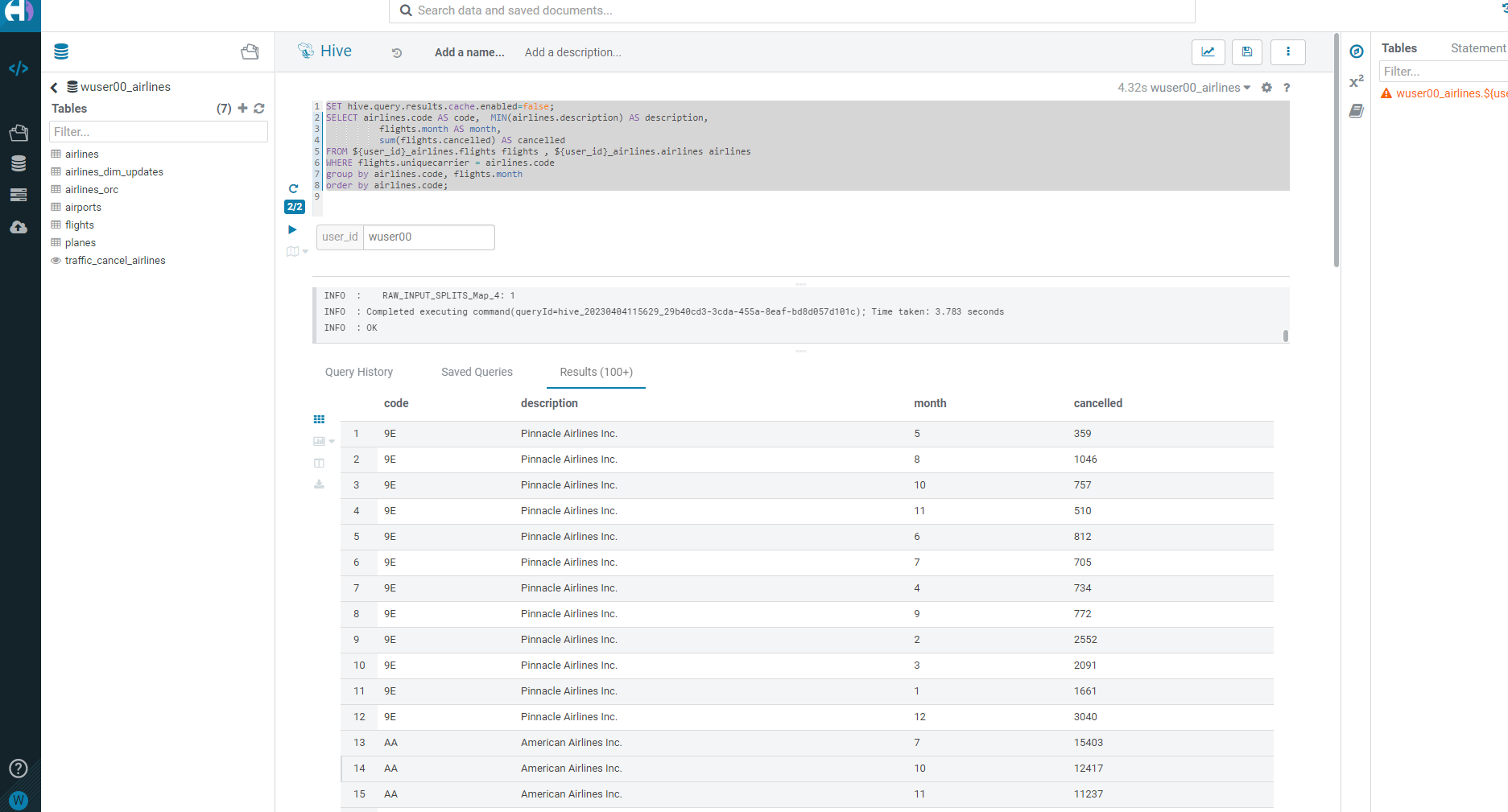
Copy/paste the following, make sure to highlight the entire block, and execute the following.
SET hive.query.results.cache.enabled=false;

drop table  if exists ${user_id}_airlines.airlines;
CREATE EXTERNAL TABLE ${user_id}_airlines.airlines (code string, description string) STORED BY ICEBERG STORED AS ORC TBLPROPERTIES ('format-version' = '2');

INSERT INTO ${user_id}_airlines.airlines SELECT * FROM ${user_id}_airlines_raw.airlines_csv;

SELECT airlines.code AS code,  MIN(airlines.description) AS description,
          flights.month AS month,
          sum(flights.cancelled) AS cancelled
FROM ${user_id}_airlines.flights flights , ${user_id}_airlines.airlines airlines
WHERE flights.uniquecarrier = airlines.code
group by airlines.code, flights.month;Note: Hive has built in performance improvements, such as a Query Cache that stores results of queries run so that similar queries don’t have to retrieve data, they can just get the results from the cache. In this step we are turning that off using the SET statement, this will ensure when we look at the query plan, we will not retrieve the data from the cache.
Note: With this query you are combining an Iceberg Table Format (flight table) with a Hive Table Format (airlines ORC table) in the same query.
-
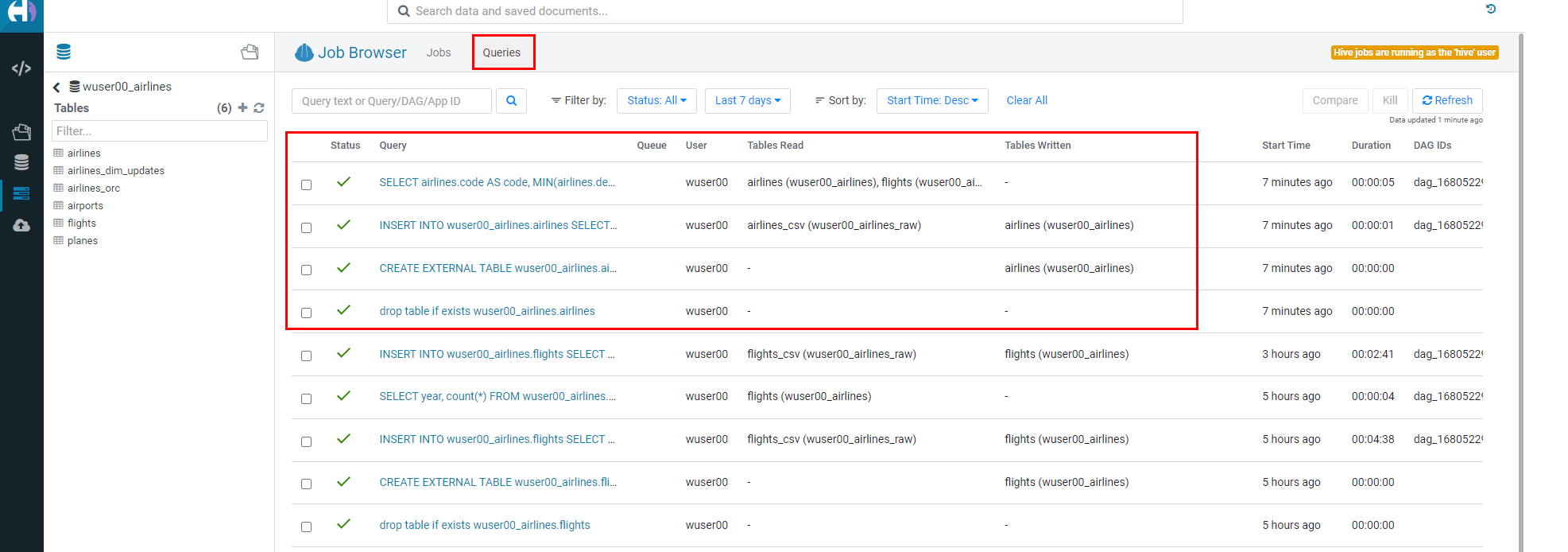
Let’s look at the Query Plan that was used to execute this query. On the left side click on
Jobs, as shown in the screenshot below.
-
Then click on
Queries. This is where an Admin will go when he wants to investigate the queries. In our case for this lab, we’d like to look at the query we just executed to see how it ran and the steps taken to execute the query. Administrators would also be able to perform other monitoring and maintenance tasks for what is running (or has been run). Monitoring and maintenance tasks could include cancel (kill) queries, see what is running, analyze whether queries that have been executed are optimized, etc.
-
Click on the first query as shown below. Make sure that this is the latest query. You can look at the `Start Time' field here to know if it’s the latest or not.

-
This is where you can analyze queries at a deep level. For this lab let’s take a look at the explain details, by clicking on
Visual Explaintab.
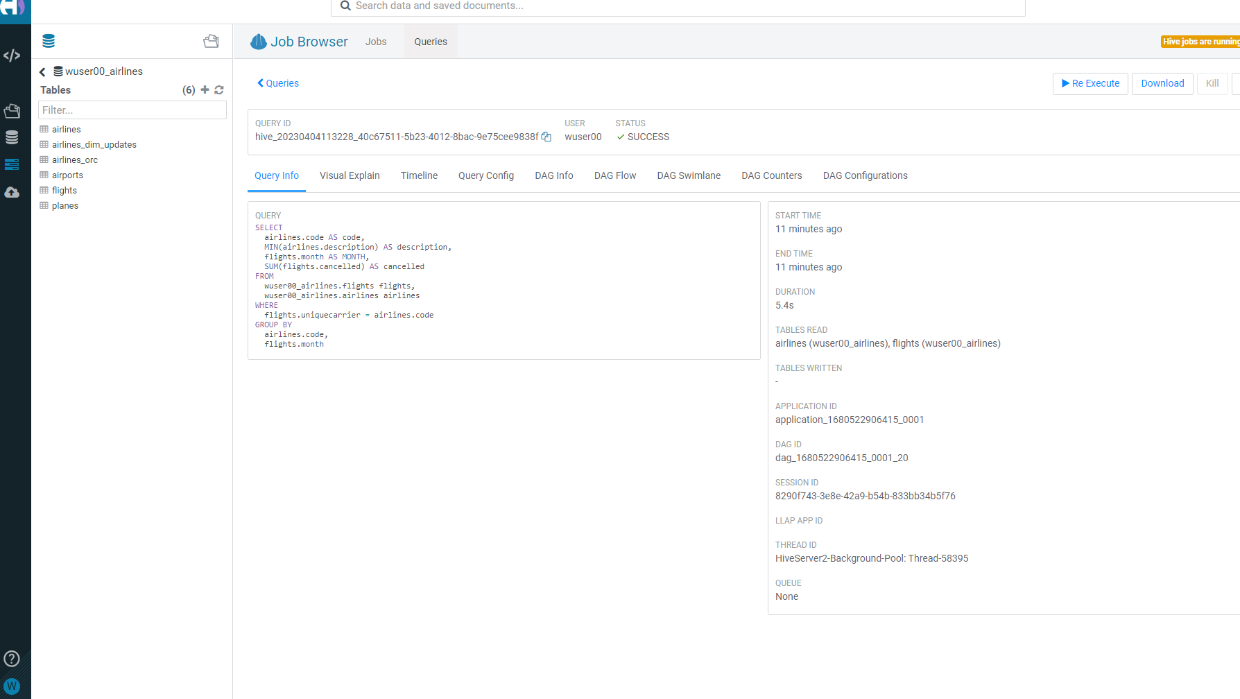
-
This plan shows that this query needs to Read
flights(86M rows) andairlines(1.5K rows) with hash join, group, and sort. This is a lot of data processing and if we run this query constantly it would be good to reduce the time this query takes to execute.
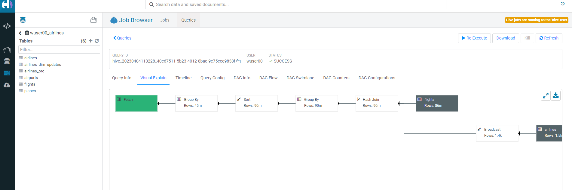
-
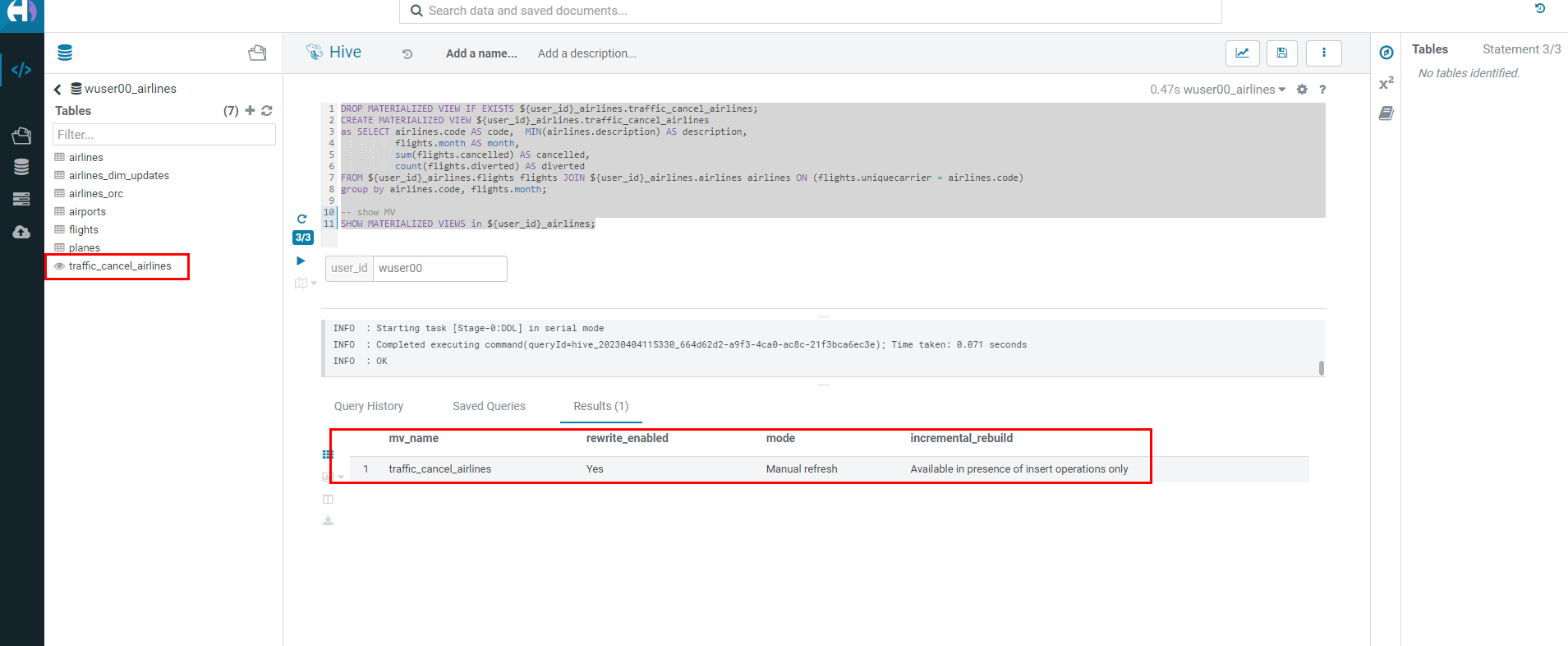
Create Materialized View (MV) - Queries will transparently be rewritten, when possible, to use the MV instead of the base tables. Copy/paste the following, highlight the entire block, and execute.
DROP MATERIALIZED VIEW IF EXISTS ${user_id}_airlines.traffic_cancel_airlines;
CREATE MATERIALIZED VIEW ${user_id}_airlines.traffic_cancel_airlines
as SELECT airlines.code AS code,  MIN(airlines.description) AS description,
          flights.month AS month,
          sum(flights.cancelled) AS cancelled,
          count(flights.diverted) AS diverted
FROM ${user_id}_airlines.flights flights JOIN ${user_id}_airlines.airlines airlines ON (flights.uniquecarrier = airlines.code)
group by airlines.code, flights.month;

-- show MV
SHOW MATERIALIZED VIEWS in ${user_id}_airlines;-
Run Dashboard Query again to see usage of the MV - Copy/paste the following, make sure to highlight the entire block, and execute the following. This time an
order bywas added to make this query must do more work.
SET hive.query.results.cache.enabled=false;
SELECT airlines.code AS code,  MIN(airlines.description) AS description,
          flights.month AS month,
          sum(flights.cancelled) AS cancelled
FROM ${user_id}_airlines.flights flights , ${user_id}_airlines.airlines airlines
WHERE flights.uniquecarrier = airlines.code
group by airlines.code, flights.month
order by airlines.code;-
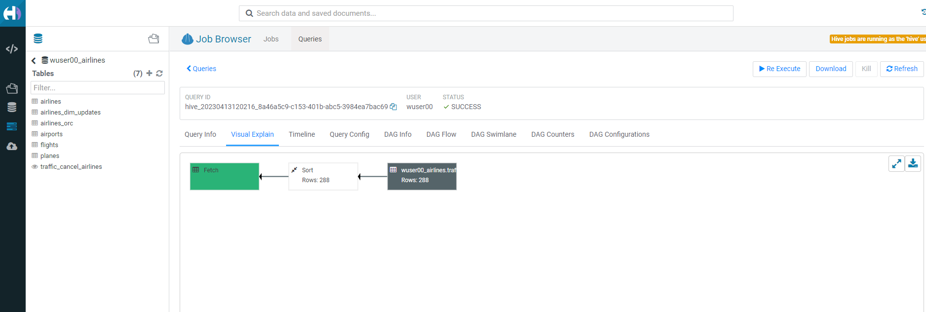
Let’s look at the Query Plan that was used to execute this query. On the left menu select
Jobs. On the Jobs Browser - select theQueriestab to the right of theJobbrowser header. Hover over & click on the Query just executed (should be the first row). Click onVisual Explaintab. With query rewrite the materialized view is used and the new plan just reads the MV and sorts the data vs. readingflights (86M rows)andairlines (1.5K rows)with hash join, group and sorts. This results in significant reduction in run time for this query.
In this step you will experience the combination of what the Data Warehouse and the Shared Data Experience (SDX) offers. SDX enables you to provide Security and Governance tooling to ensure that you will be able to manage what is in the CDP Platform without having to stitch together multiple tools. Read more about SDX by clicking here.
-
Go to the Cloudera Data Platform Console and click on Data Catalog
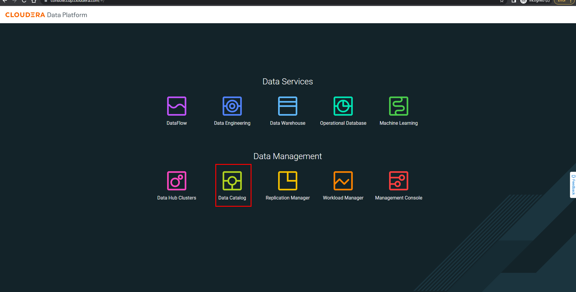
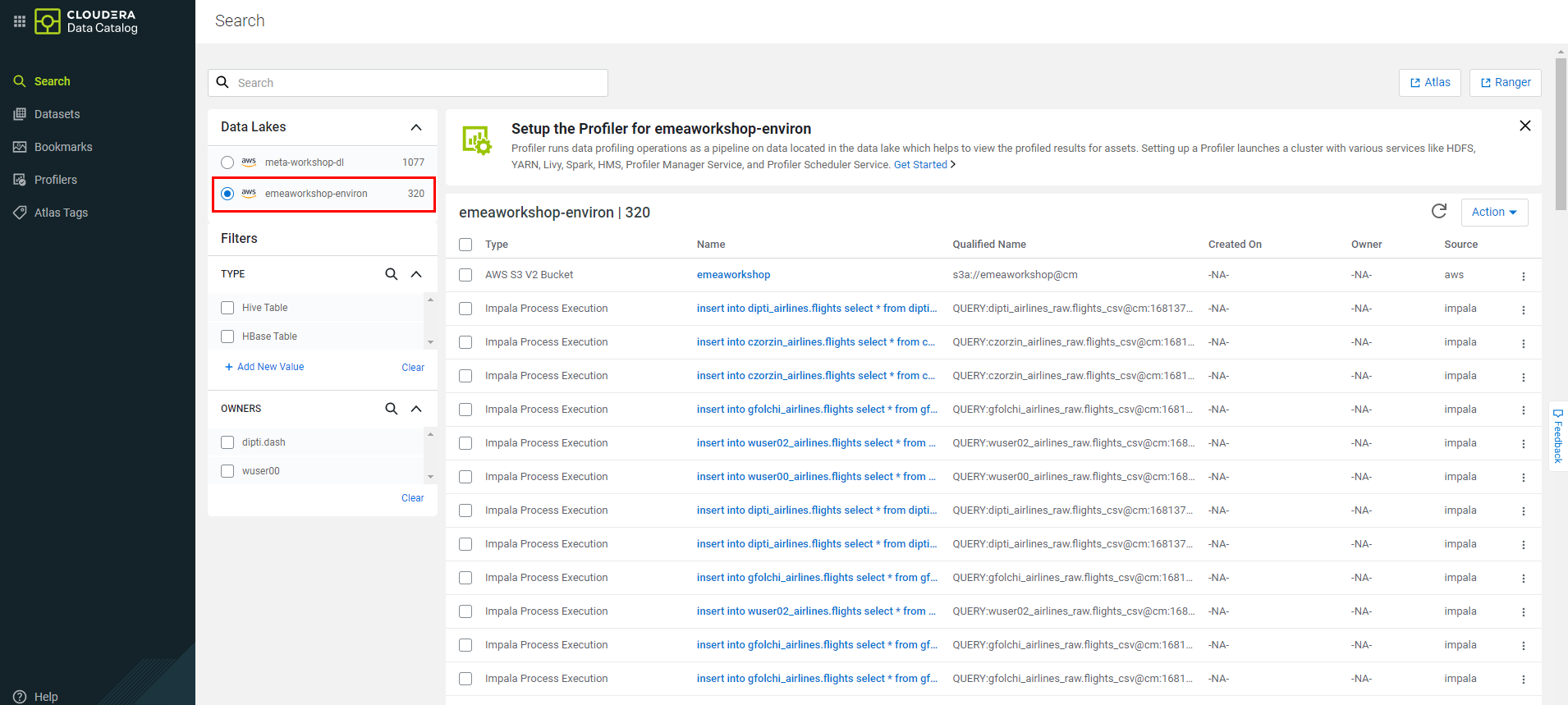
-
Change the radio button to select appropriate data lake. In this case it is
emeaworkshop-environ.
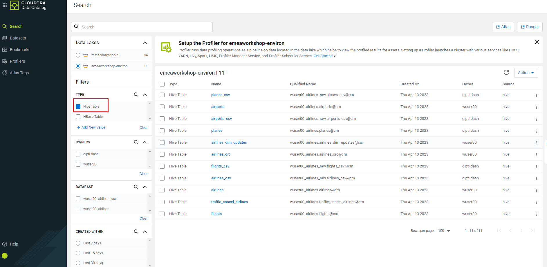
-
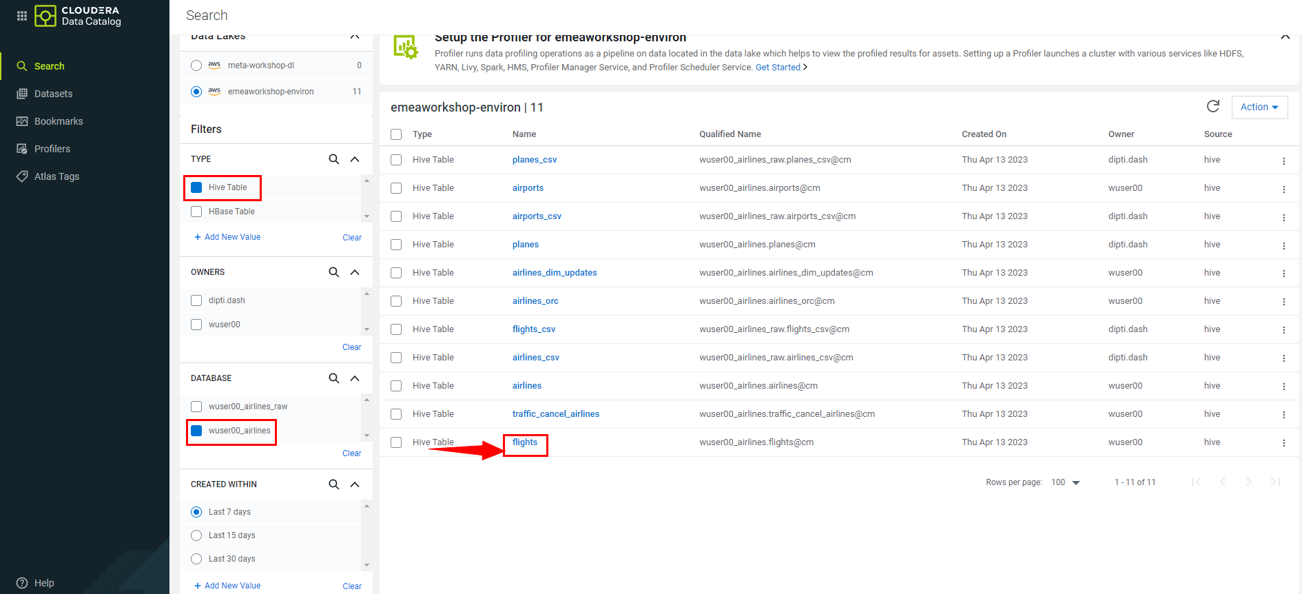
Filter for Assets we created - below the Data Lakes on the left of the screen under Filters, select
TYPEto beHive Table. The right side of the screen will update to reflect this selection.
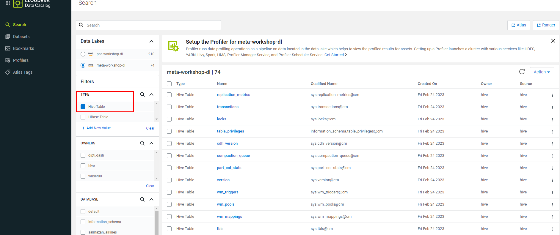
-
Under
DATABASE, clickAdd new Value. In the box that appears start typing your<user_id>when you see the<user_id>_airlinesdatabase pop up select it.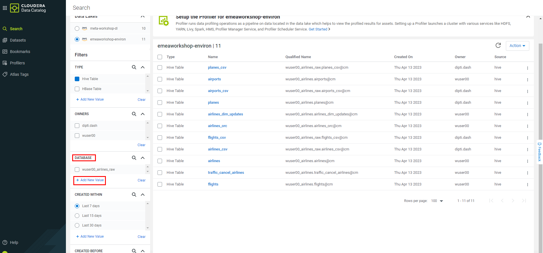
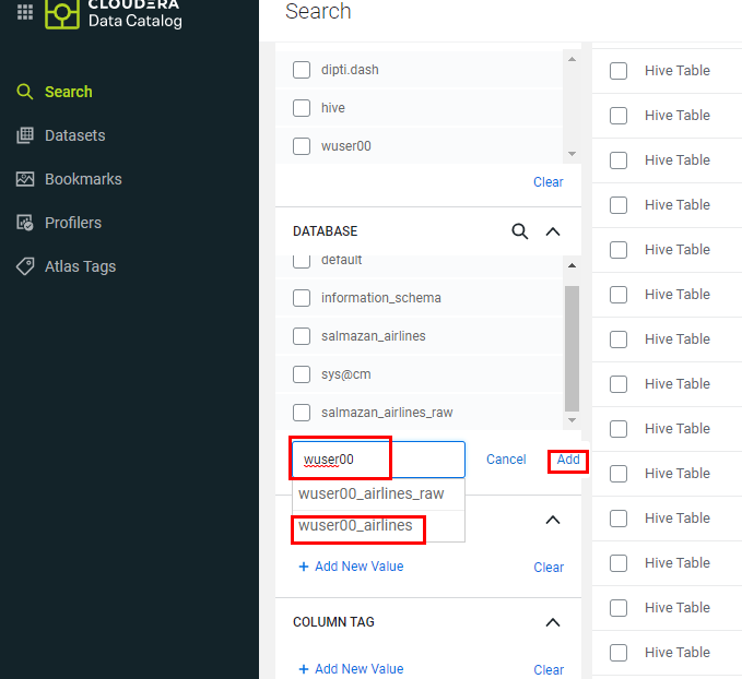
-
You should now see the tables and materialized views that have been created in the
<user_id>_airlinesdatabase. Click onflightsin theNamecolumn to view more details on the table.
-
This page shows information about the
flightstable such as the table owner, when the table was created, when it was last accessed, and other properties. Below the summary details is the Overview tab which shows the lineage - hover over the flights click on the “i” icon that appears to see more detail on this table.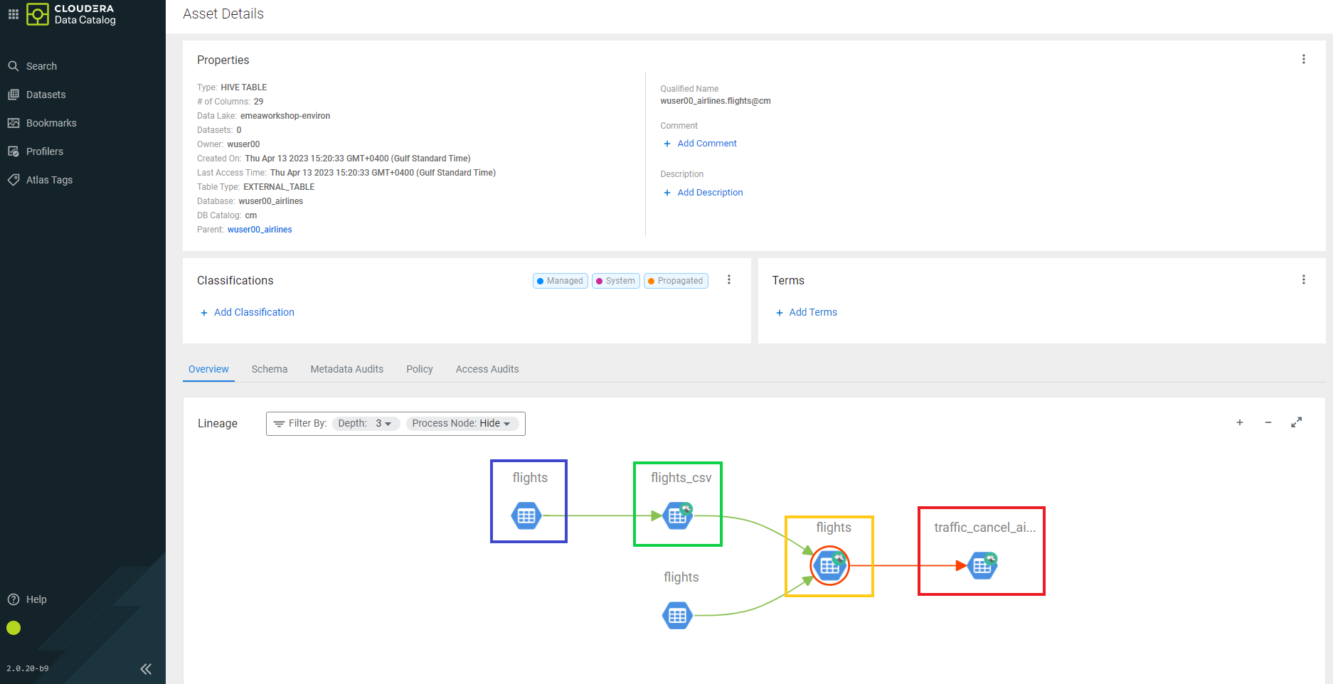
The lineage shows:
[blue box] - flights data file residing in an s3 folder.
[green box] - is showing how the flights_csv Hive table is created, this table was created and points to the data location of flights (blue box) s3 folder.
[orange box]- is showing the flights Iceberg table and how it is created, it uses data from flights_csv Hive table (CTAS).
[red box] - traffic_cancel_airlines is a Materialized View that uses data from the flights Iceberg table.
-
Click on the Policy tab to see what security policies have been applied on this table. Click on the arrow next
all - database, tablePolicy Nameto the number as shown in the screenshot+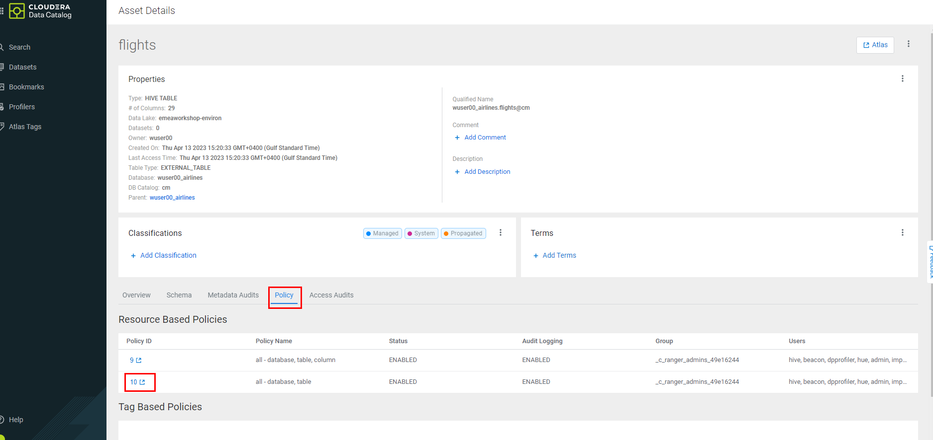
-
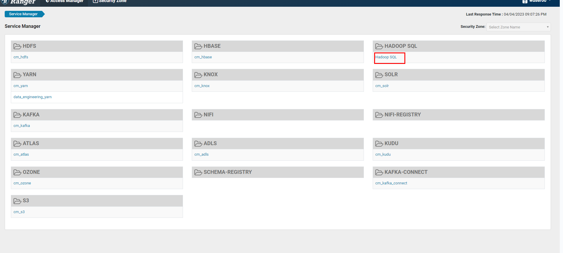
It will open
Rangerwhich is for access management. Using Security (Ranger) - we can modify and create security policies for the various CDP Data Services. Click onHadoop SQLlink in the upper right corner - to view the security policies in place for CDW. Here, will stick to the CDW related security features.
-
This screen shows the general Access related security policies - who has access to which Data Lakehouse databases, tables, views, etc. Click on the
Row Level Filtertab to see the policies to restrict access to portions of data.
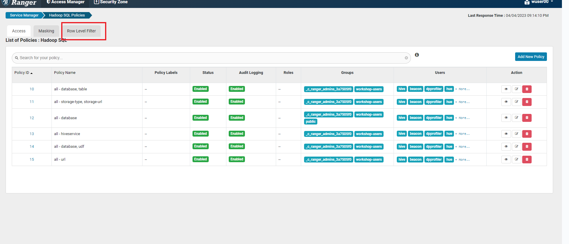

-
There are currently no policies defined. Click on the
Add New Policybutton on top right corner.

-
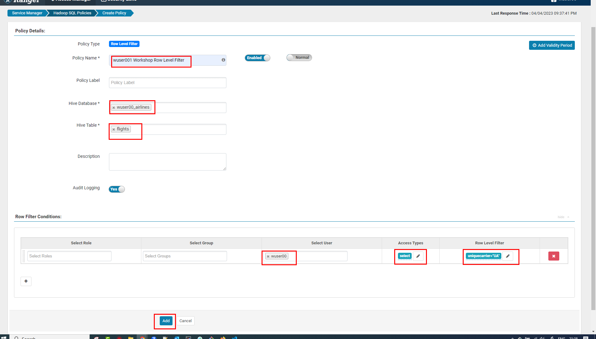
Fill out the form as follows.
Policy Name: <user_id>_RowLevelFilter (Ex: wuser00_RowLevelFilter)
Hive Database: <user_id>_airlines (Ex: wuser00_airlines)
Hive Table: flights (start typing, once you see this table in the list, select it)
Row Filtering Conditions:
(a)Select User: <user_id>
(b)Access Types: select
(c)Row Level Filter: uniquecarrier="UA"
Click Add button to accept this Policy.
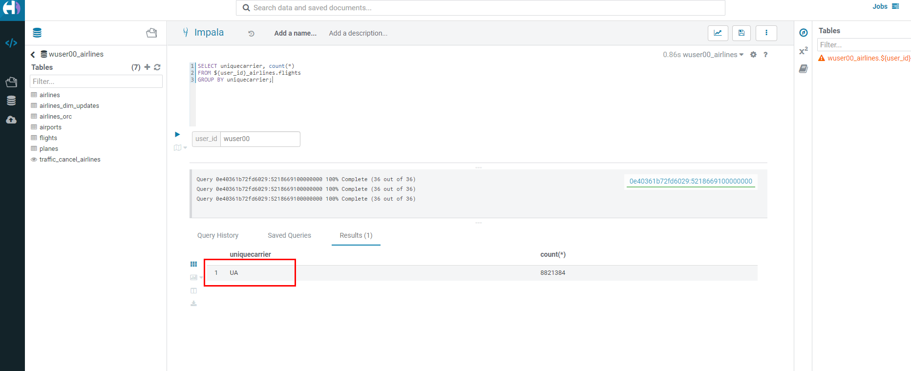
SELECT uniquecarrier, count(*)
FROM ${user_id}_airlines.flights
GROUP BY uniquecarrier;In this step you will build a Logistics Dashboard using Cloudera Data Visualization. The Dashboard will include details about flight delays and cancellations. But first we will start with Data Modeling.
-
If you are not on the CDP home page, then go there and click on the following CDW icon to go into Cloudera Data Warehouse.
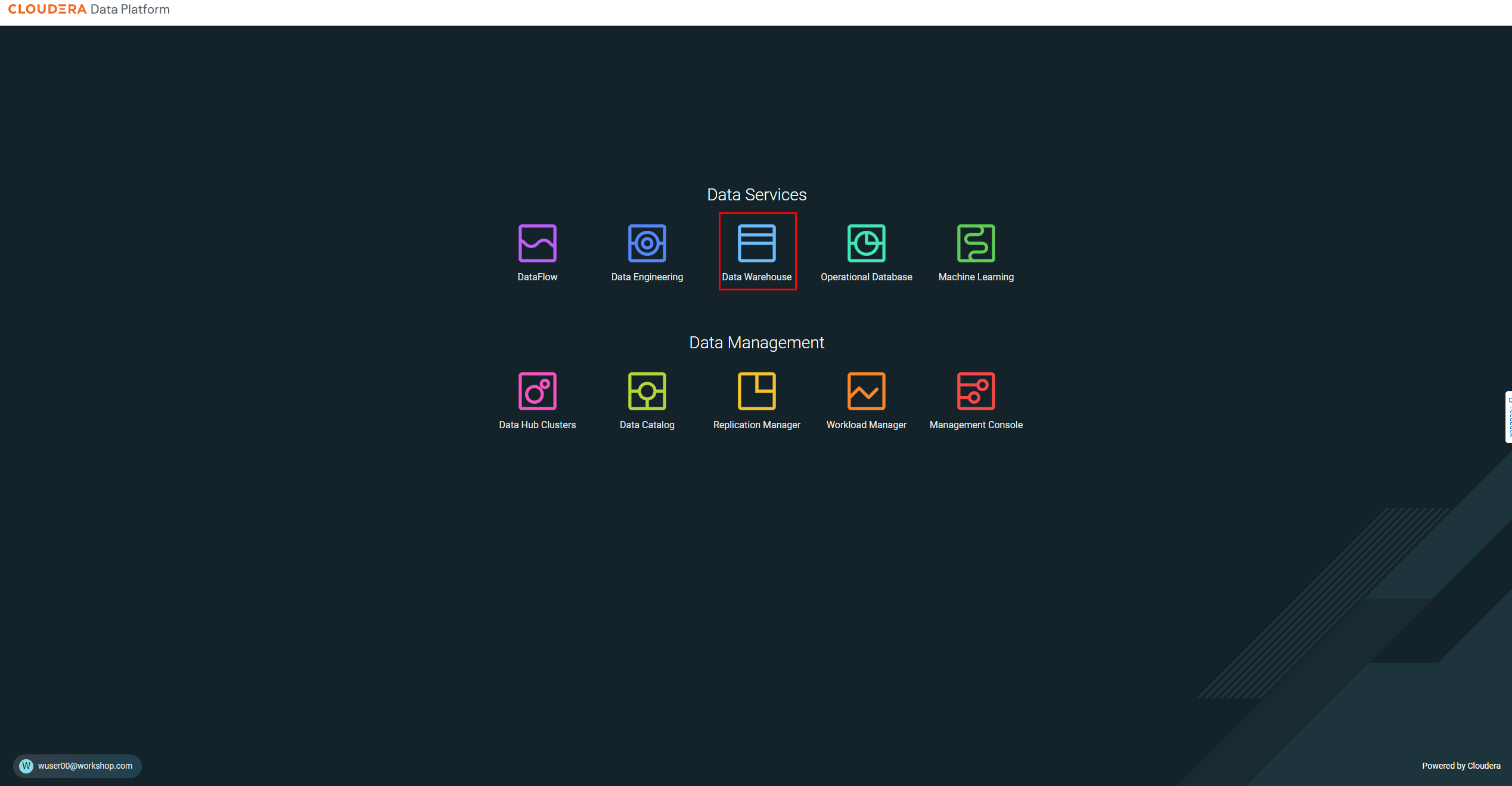
-
Then click on
Data Visualizationoption in the left windowpane. You’ll see an optionData VIZnext to the data-viz application with the nameemeaworkshop-dataviz. It should open a new window.+
-
There are 4 areas of CDV -
HOME, SQL, VISUALS, DATA- these are the tabs at the top of the screen in the black bar to the right of the Cloudera Data Visualization banner.
-
Build a Dataset (aka. Metadata Layer or Data Model) - click on
DATAin the top banner. A Dataset is a Semantic Layer where you can create a business view on top of the data - data is not copied; this is just a logical layer.

-
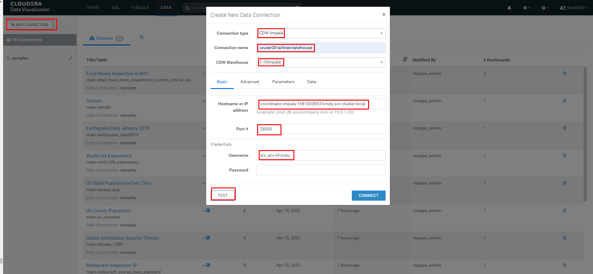
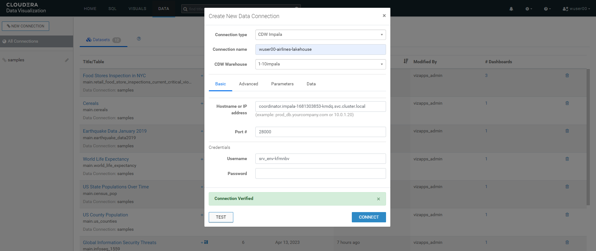
Create a connection - click on the NEW CONNECTION button on the left menu. Enter the details as shown in the screenshot and click on
TEST.
Connection type: SelectCDW Impala.
Connection name:<user_id>-airlines-lakehouse(Ex-wuser00-airlines-lakehouse).
CDW Warehouse:Make Sure you select the warehouse that is associated with your <user_id>.
Hostname or IP address: Gets automatically selected.
Port:Gets automatically filled up.
Username:Gets automatically filled up.
Passowrd:Blank
-
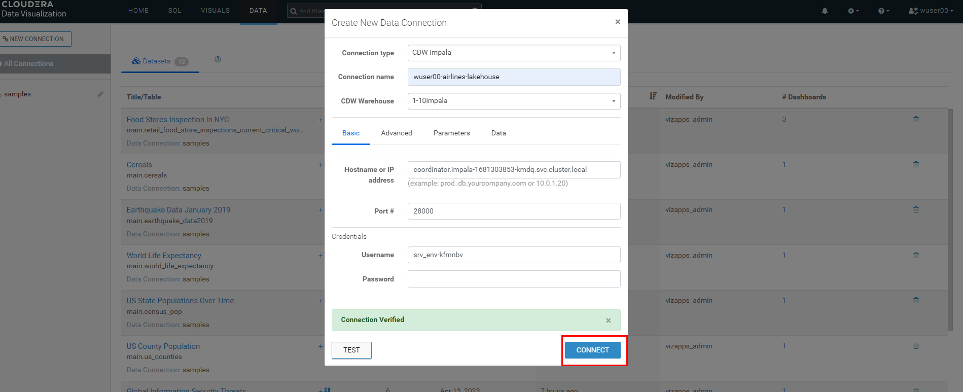
You will see your connection in the list of connections on the left menu. On the right side of the screen you will see Datasets and the Connection Explorer. Click on
NEW DATASET.


-
Fill the details as following and click
CREATE.airline_logisticsgets created
Dataset title -airline_logistics.
Dataset Source - SelectFrom Table(however, you could choose to directly enter a SQL statement instead).
Select Database -<user_id>_airlines(Make Sure you select the database that is associated with your <user_id>).
Select Table -flights.
-
Edit the Dataset - click on
airline_logisticson the right of the screen. This will open the details page, showing you information about the Dataset, such as connection details, and options that are set. Click onFieldsoption in the left window pane.


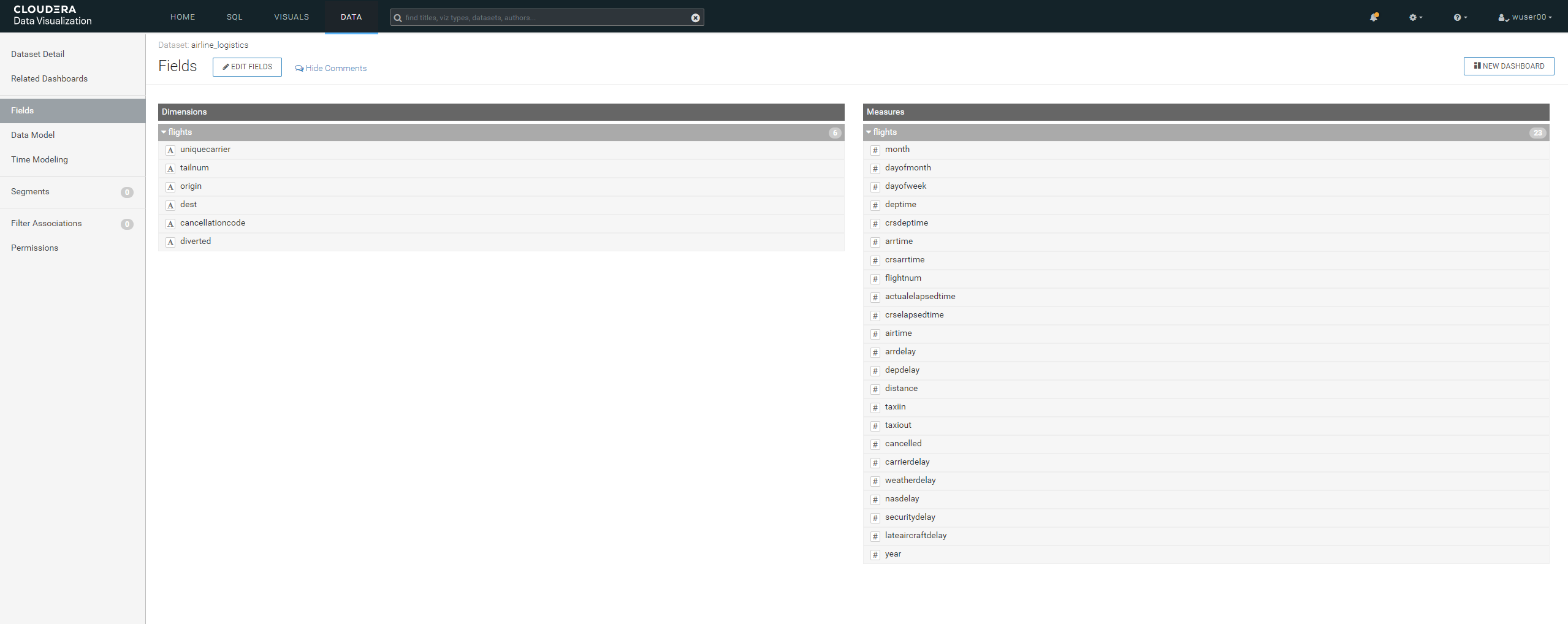
-
Click on
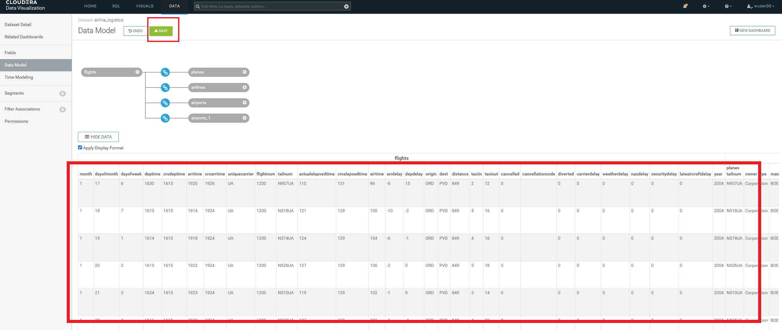
Data Model- for our Dataset we need to join additional data to the flights table including theplanes,airlines, andairportstables.
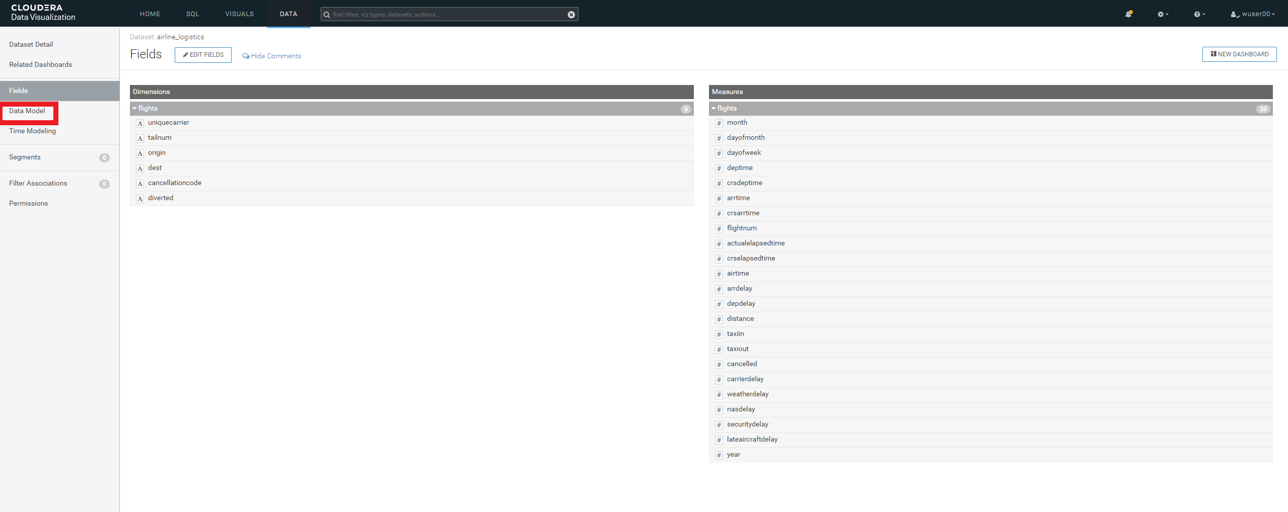
-
Select the appropriate
Database Namebase on your user id (Ex:wuser00_airlines) and table nameplanes.
-
Then click on the

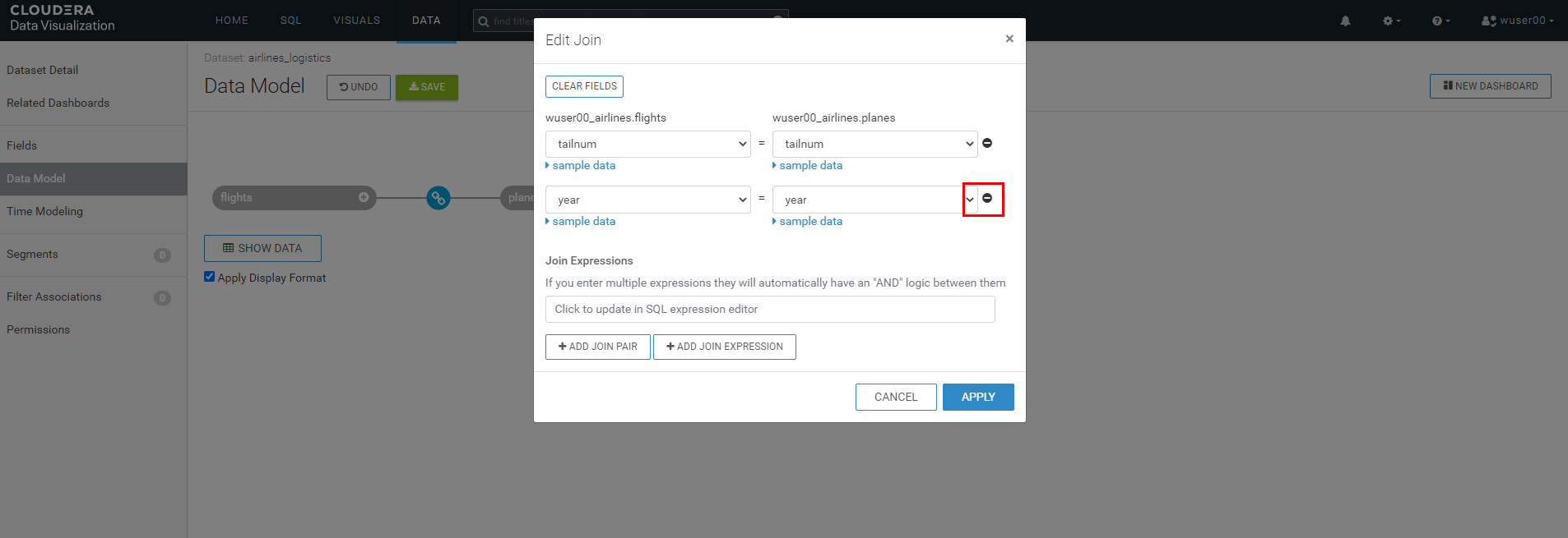
joinicon and see that there are 2 join optionstailnum&year. Click onEDIT JOINand then remove theyearjoin by clicking little-(minus) icon to the right next to theyearcolumn. Click onAPPLY.




-
Now we will create join between another table. Click on
+icon next toflightsas shown below. Select the appropriateDatabase Namebased on your <user_id> (Ex:wuser00_airlines) and table nameairlines.


-
Make sure you select the column
uniquecarrierfromflightsand columncodefromairlinestable. ClickAPPLY.


-
Click on
+icon next toflightsas shown below. Select the appropriateDatabase Namebased on your <user_id> (Ex:wuser00_airlines) and table nameairports.

-
Make sure you select the column
originfromflightsand columniatafromairportstable. ClickAPPLY.

-
Click on
+icon next toflightsas shown below. Select the appropriateDatabase Namebased on your <user_id> (Ex:wuser00_airlines) and table nameairports.

-
Make sure you select the column
destfromflightsand columniatafromairportstable. ClickAPPLY. Then click onSAVE.


-
Verify that you have the joins which are as following. You can do so by clicking the

joinicon.
flights.tailnum—planes.tailnum
flights.uniquecarrier—airlines.code
flights.origin—airports.iata
flights.dest—airports_1.iata -
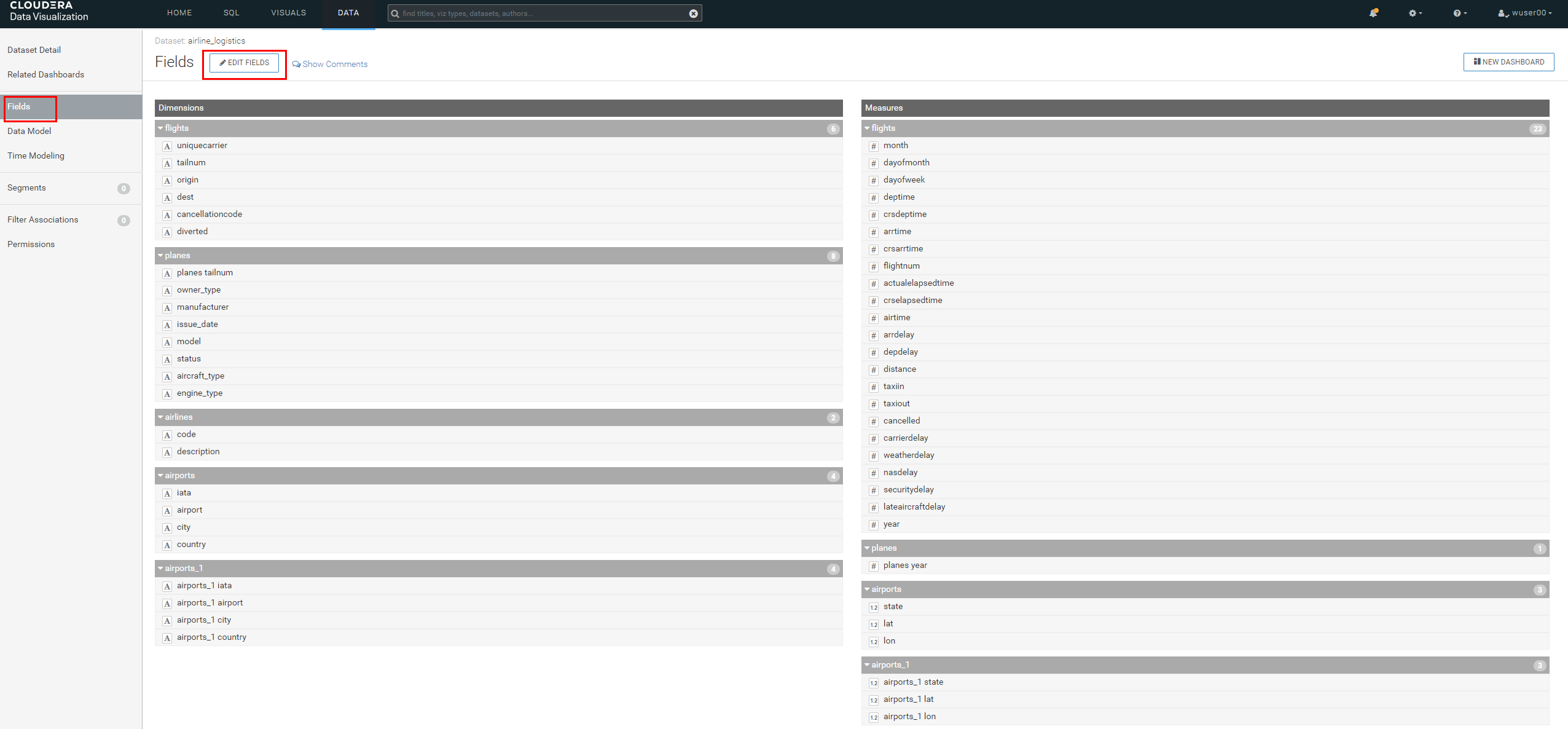
Click on
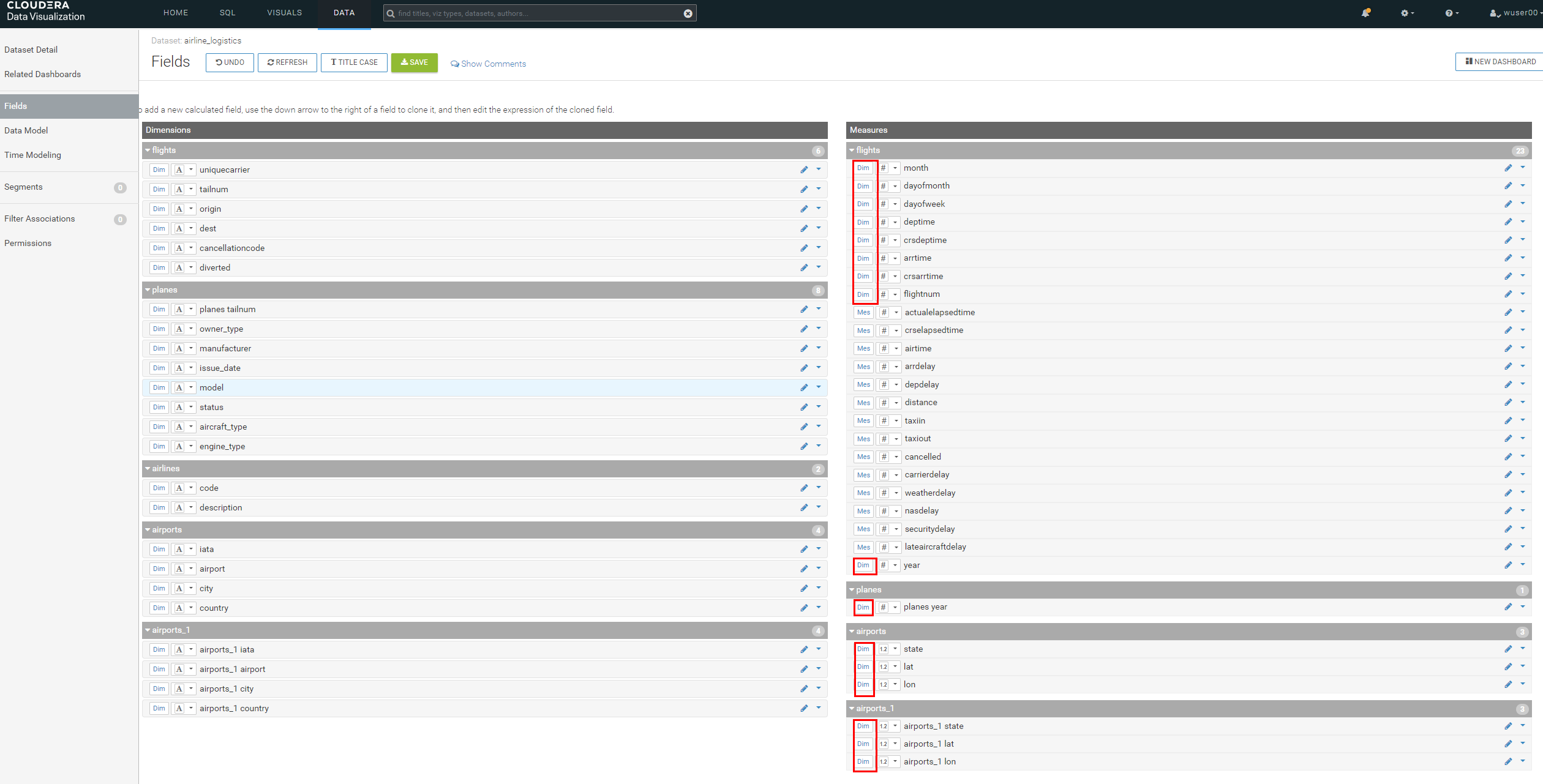
Fieldscolumn on the left window pane. Then click onEDIT FIELDS. Make sure that you click on the highlighted area to change#(measures icon) next to each column toDim(dimension icon). The columns are as following.-
flightstable: Columns (month,dayofmonth,dayofweek,deptime,crsdeptime,arrtime,crsarrtime,flightnum&year) -
planestable:All columns -
airportstable:All columns -
airports_1table:All columns
-
-
Click on
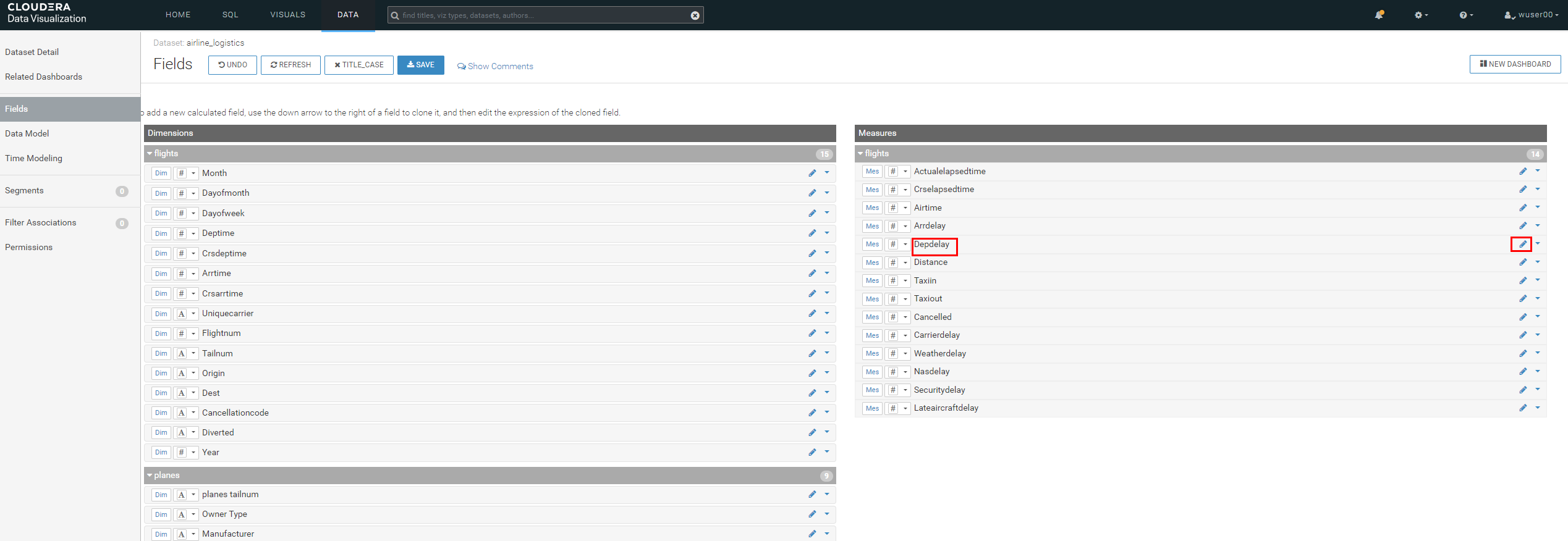
TITLE CASE. And notice that the column names changes to beCamel case. Click on thepencilicon next toDepdelayicon.

-
Change the
Default AggregationtoAverage. Click on theDisplay Formatand then changeCategoryto beInteger. Check mark the box next theUse 1000 separator. Click onAPPLY.


-
Click on
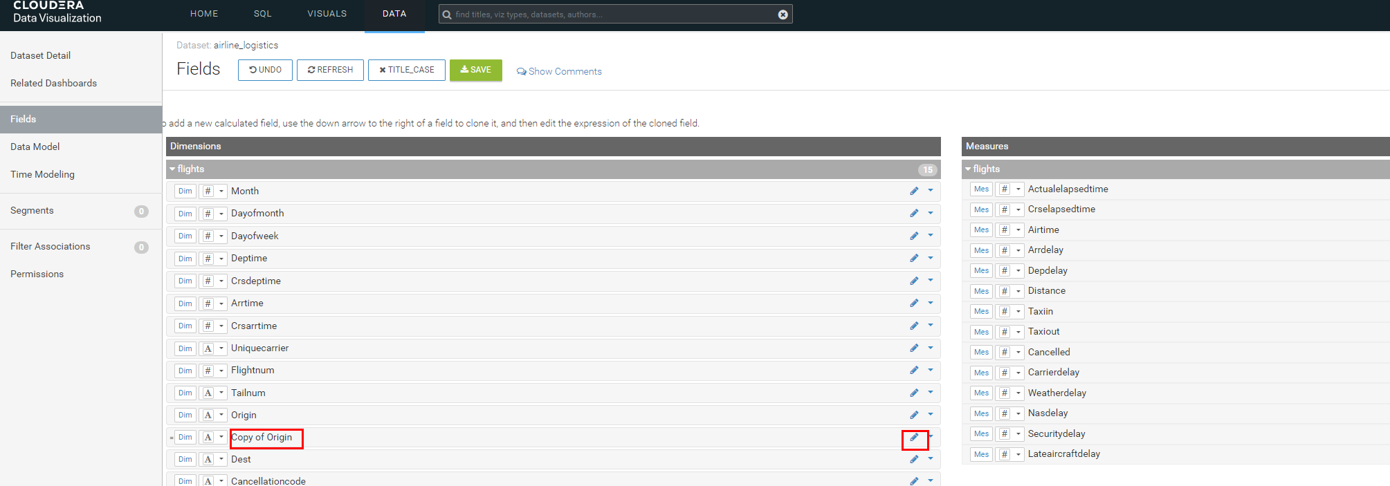
down arrowshown against theOrigincolumn and the click onClone. A columnCopy of Originis created. Click on the 'pencil' icon next to it.

-
Change the
Display NametoRoute. Then click onExpressionand enter the following in theExpressioneditor. Click onAPPLY.
concat([Origin], '-', [Dest])
-
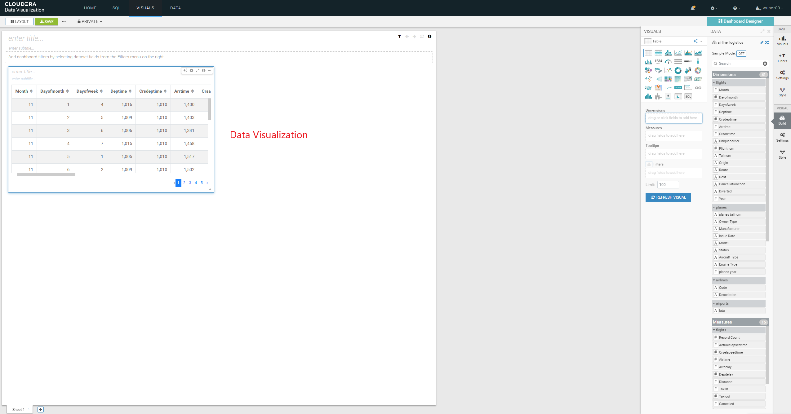
Now we will create a dashboard page to based on the data model that we just created. Click on
NEW DASHBOARD.
-
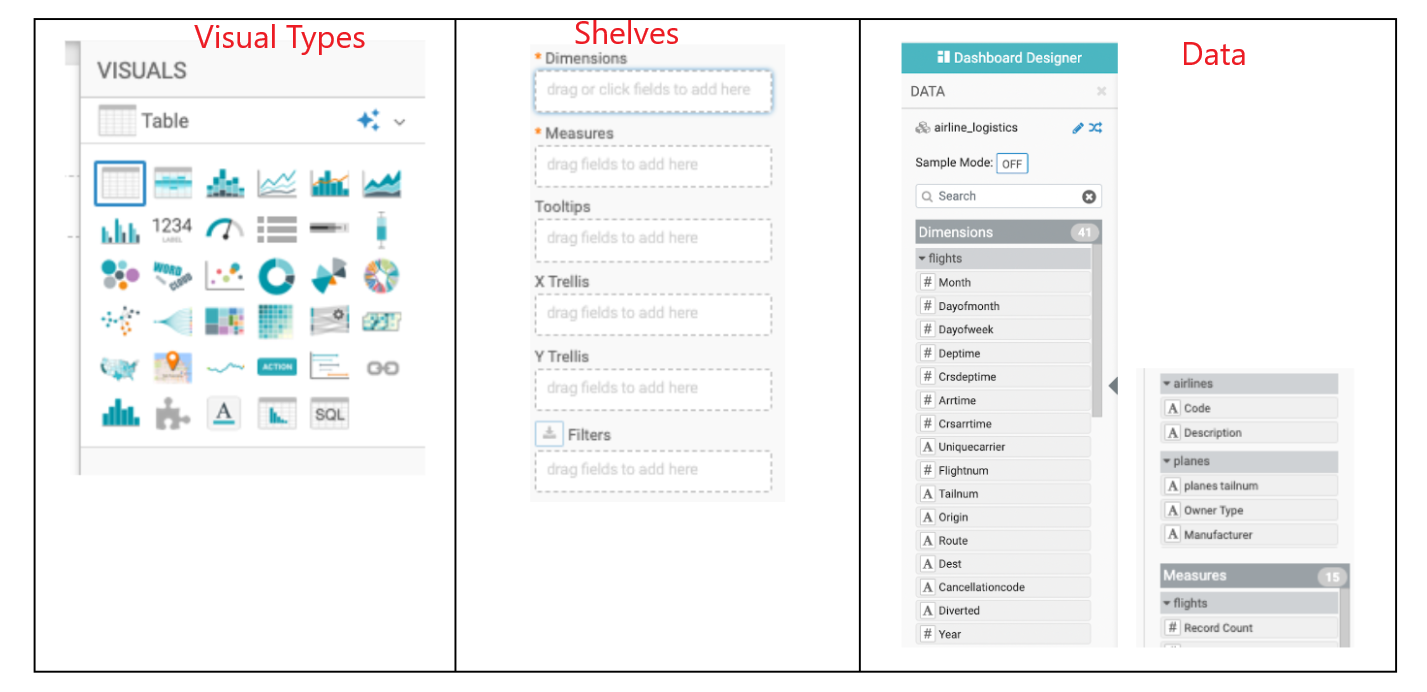
A quick overview of the screen that you are seeing is as following. On the right side of the screen there will be a VISUALS menu. At the top of this menu, there is a series of Visual Types to choose from. There will be 30+ various visuals to choose from. Below the Visual Types you will see what are called Shelves. The Shelves that are present depend on the Visual Type that is selected. Shelves with a
*are required, all other Shelves are optional. On the far right of the page there is a DATA menu, which identifies the Connection & Dataset used for this visual. Underneath that is the Fields from the Dataset broken down by Dimensions and Measures. With each of these Categories you can see that it is subdivided by each Table in the Dataset.
-
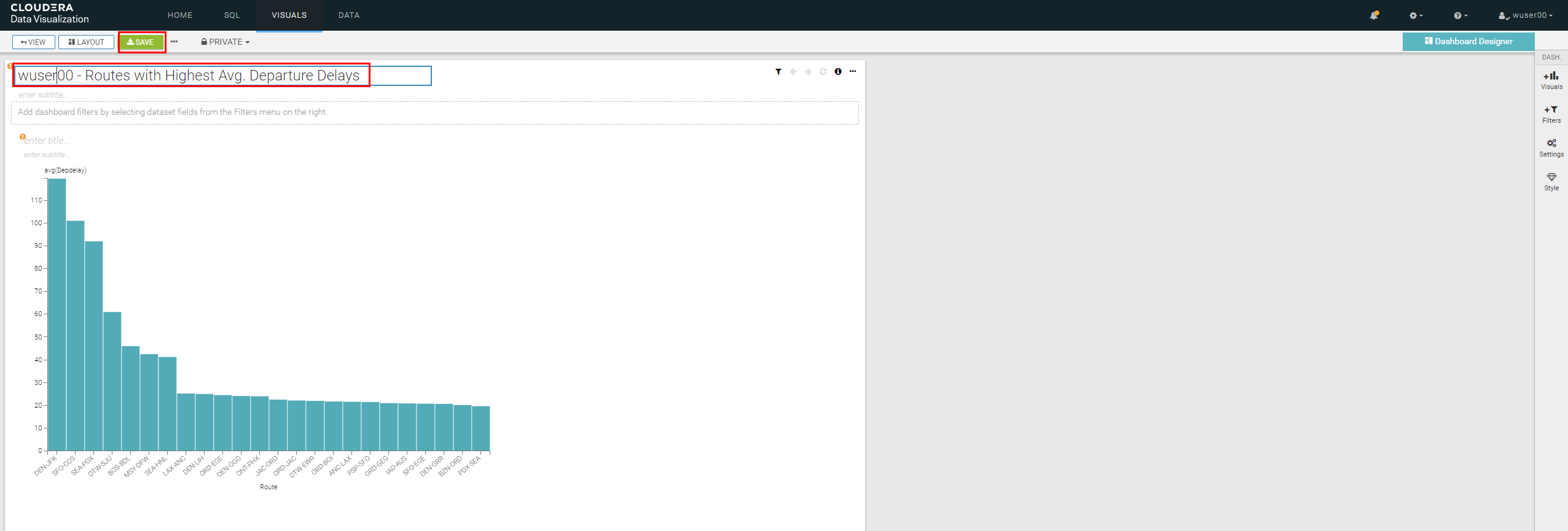
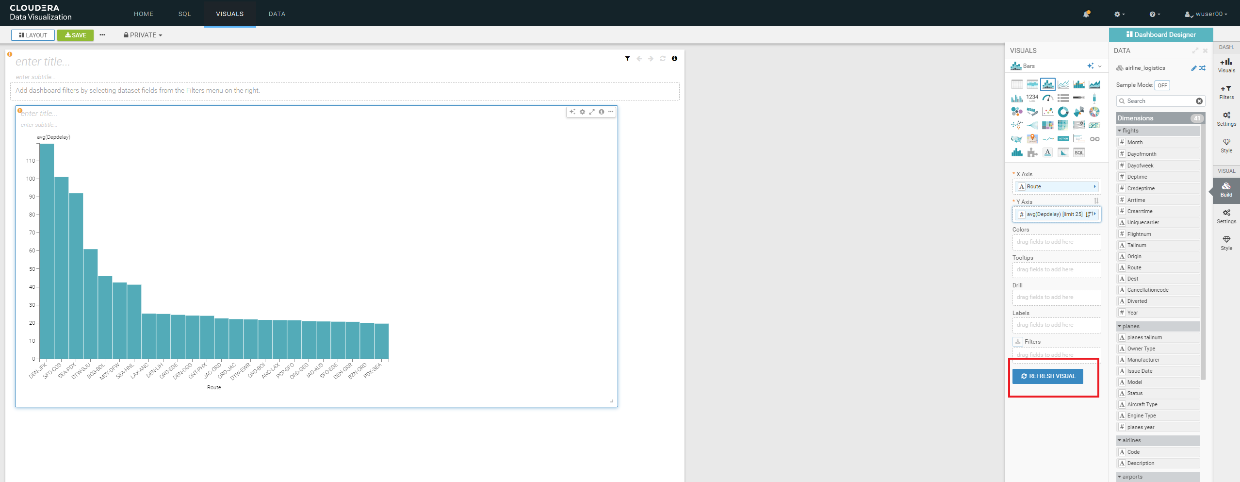
Let’s build 1st visual -
Top 25 Routes by Avg Departure Delay. CDV will add a Table visual displaying a sample of the data from the Dataset as the default visualization when you create a new Dashboard or new Visuals on the Dashboard (see New Dashboard screen above). The next step is to modify (Edit) the default visualization to suit your needs. -
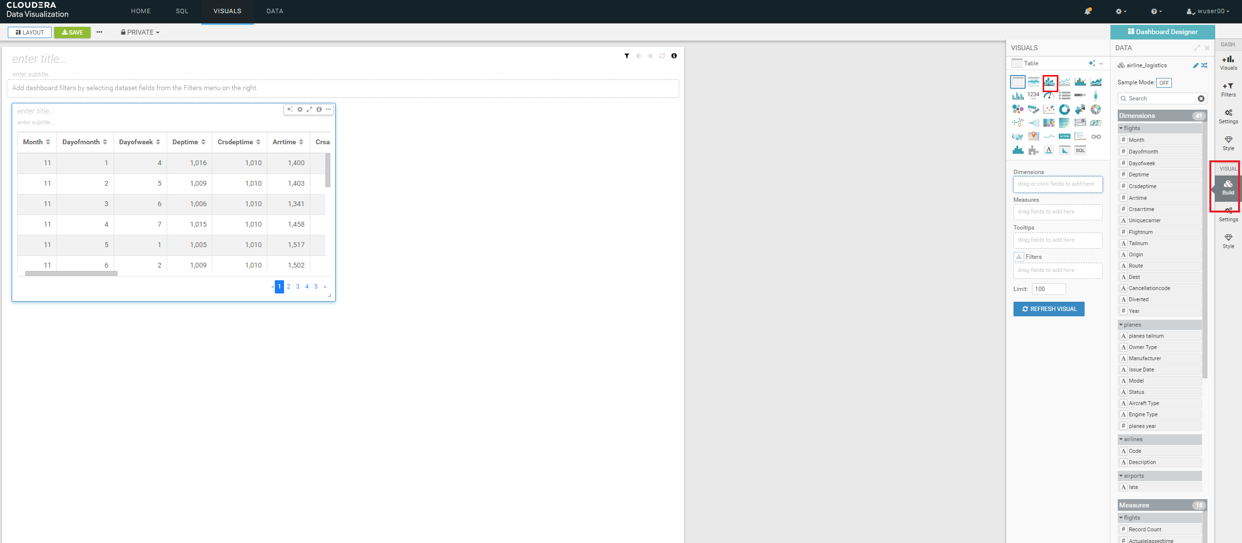
Pick the Visual Type - Select the
Stacked Barchart visual on the top right as shown below. Make sureBuildis selected for it to appear in the right side.
-
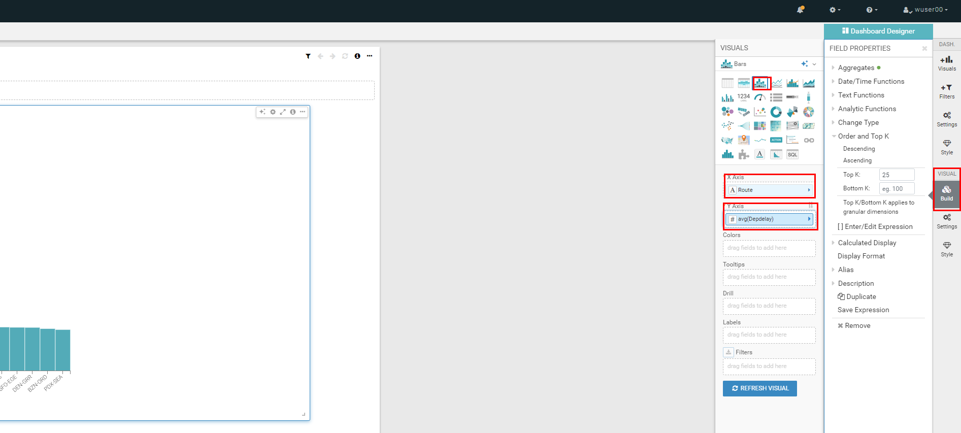
Find
RouteunderDimensions → flights. Drag toX-Axis. Similarly, findDepDelayunderMeasures → flights. Drag toY-Axis. By default the aggergation selected is average and hence you would seeavg(Depdelay).
-
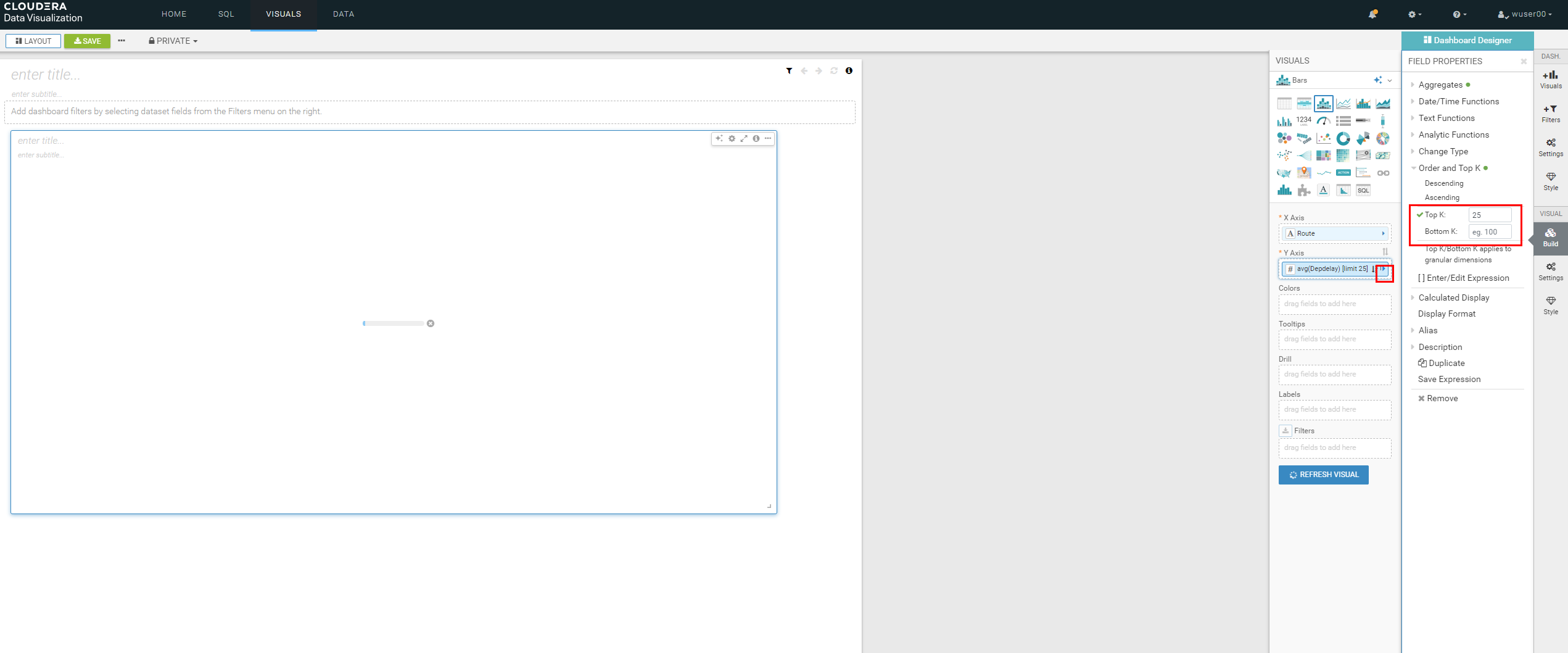
Click on the arrow next to
avg(Depdelay). Enter25against the text box labeledTop K. Click onREFRESH VISUAL.
-
Click
enter titleand enter the title based on your user id as -<user_id>- Routes with Highest Avg. Departure Delays. Then click onSAVE.