Dynamic Programming and Optimal Control

by : walkerchi

Mathematics

Notation

$x$ : state, $x\in\mathcal S = \mathcal S^+\cup{0}$,
- $x_0$ or $x(0)$ : initial state for discrete / continuous situation
- there are $N_x$ distinct states for each time step
- $\tilde x$ tend to represent extend states like $\tilde x_k = \begin{bmatrix}x_k,y_k\end{bmatrix}^\top$
$w(t)$ : disturbance
$u(t)$ : control input , $u\in\mathcal U$, there are $N_u$ distinct control inputs for each time step
$\mu(t,x)$ : admissible control law (policy), $u(t)\sim \mu(t,x)$
- $\pi$ : policy, $\pi^*$ optimal policy
$f(x,u)$ : system evolution
- for continuous system: $\dot x(\tau)=f(x(\tau),u(\tau))$
- for discrete system : $x_{k+1}= f_k(x_k,u_k,w_k)$
$g_k(x,u)$ : cost for each step ,
- $g_N(x)$ is the cost for discrete terminal state
- $h(x)$ is the cost for continuous terminal state
$J(t,x)$ : cost function, $J^*$ optimal policy
$N$ : time horizon
$P_{ij}$ : probability of transition from state $i$ to state $j$, $\text{Pr}(x_{k+1}=j|x_k=i,u_k=\mu(i)) = P_{ij}(\mu(i))$
$q(i,u)$ : expectation of cost $q(i,u)=\underset{w|x=i,u=\text u}{\mathbb E}[g(x,u,w)]$
$p(t)$ : trajectory

Probability

$x\sim\mathcal N(\mu,\sigma^2)$ then $x^2\sim\mathcal N(\mu^2+\sigma^2, 2\sigma^4+4\mu^2\sigma^2)$
$x\sim \mathcal N(\mu, \sigma^2)$ then $Cx \sim \mathcal N(C\mu, C^2\sigma^2)$

Quadratic

$f(x) = ax^2+bx+c$

$f'(x)=0\to x = -\frac{b}{2a}$
$f(x)|_{f'(x)=0} = -\frac{b^2}{4a}+c$

Laplace Transform

time domain	$s$ domain
$1$	$\frac{1}{s}$
$e^{at}$	$\frac{1}{s-a}$
$\dot f$	$sF - f(0)$
$e^{at}f$	$F(s-a)$
$f(at)$	$\frac{1}{a}F(\frac{s}{a})$
$af+bg$	$aF+bG$

Problem Statement

Dynamics $$ x_{k+1} = f_k(x_k,u_k,w_k)\ \dot x = f(x,u,w) $$ Cost $$ J_\pi = \mathbb E\left[g_N + \sum_{k=0}^{N-1}g_k(x_k,u_k,w_k)\right] $$

$J^\pi$ : optimal cost $J\pi^ = \text{max}~J_\pi$

Open Loop : control inputs are determined at beginning

expected cost

$$ J(\text x) = \underset{(X_1,W_0|x_0=\text x)}{\mathbb E}\left[g_N(x_N) + \sum_{k=0}^{N-1}g_k(x_k,\bar u_k,w_k)\right] $$

Number of Open Loop Strategies : $N_u^N$ all the possible path from start to end

Closed Loop : $u(t)\to \mu(t,x)$ control inputs depend on the measured state

expected cost

$$ J_\pi (\text x) = \underset{(X_1,W_0|x_0=\text x)}{\mathbb E}\left[g_N(x_N) +\sum_{k=0}^{N-1}g_k(x_k,\mu_k(x_k),w_k)\right] $$

Number of Close Loop Strategies : $N_u(N_u^{N_x})^{N-1}$ (number of state stay constant) or $N_u^{\sum_k N_x^k}$ all possible path for unique set of all reachable states $\sum_k N_x^k$

Open Loop vs Closed Loop

open loop is special case of closed loop
open never performs better than closed loop
for deterministic problem , closed loop is not efficient as open loop

[DPA]Dynamic Programming Algorithm

$$ J_k(\text x) = \underset{\text u\in\mathcal U(\text x)}{\text{min}} \underset{(w_k|x_k=\text x, u_k=\text u)}{\mathbb E}\left[g_k(x_k,u_k,w_k)+J_{k+1}(f(x_k,u_k,w_k))\right]\quad J_N(\text x) = g_N(\text x) $$

Number of Minimizations : number of reachable states $\sum_k N_x^k$
when there is no disturbance $w_k$, it can be solved by forward DPA

general state :

Example : $x_{k+1} = f_k(x_k,x_{k-1},u_k,u_{k-1},w_k)$, $\tilde x_{k+1} = \begin{pmatrix}x_{k+1}\y_{k+1}\s_{k+1} \end{pmatrix}=\begin{pmatrix}f_k(x_k,y_k,u_k,s_k,w_k)\y_k\u_k\end{pmatrix}$ where $y_k = x_{k-1}$, $s_k = u_{k-1}$

Infinite Horizon Problems : $N\to \infin$ and time invariant cost $g_k\to g$

Recursion $$ J_k(\text x) = \underset{\text u\in\mathcal U(\text x)}{\text{min}} \underset{(w|x=\text x, u=\text u)}{\mathbb E}\left[g(x,u,w)+J_{k+1}(f(x,u,w))\right]\quad J_N(\text x) = g_N(\text x) $$
$N\to\infin$ it becomes BE, if $J_N$ converge, then $J(x)=J^*(x)$

[BE]Bellman Equation

$$ J^(x) = \underset{u\in\mathcal U(x)}{\text{min}}\underset{(w|x=\text x,u=\text u)}{\mathbb E}[g(x,u,w)+J^(f(x,u,w))] $$ $$ V^(x) = \underset{u\in \mathcal U}{\text{min/max}}\left[r(x,u) + \alpha\sum_{x'} P_{x,x'}(u)V(x')\right] $$

convergence of IHP

[SSP]Stochastic Shortest Path : the transition from state $i$ to state $j$ is governed by $\text{Pr}(w_{k+1}=j|x_k=i,u_k=\text u)=P_{ij}$ $$ J_k(i) = \underset{\text u\in \mathcal U(i)}{\text{min}}\left(q(i,u) + \sum_{j=0}^n P_{ij}(u)J_{k+1}(j)\right) $$

$P_{ij}$ is time-invariant, $P_{ij}\ge0$
cost-free terminal state $P_{00}(\text u)=1$ and $g(0,\text u,0)=0$ $\forall \text u\in \mathcal U(0)$
In the terminal state, any admissible control action is optimal

[VI] Value Iteration $$ V_{l+1}(i) = \underset{\text u\in \mathcal U(i)}{\text{min}}\left(q(i,u) + \alpha\sum_{j=1}^n P_{ij}(\text u)V_l(j)\right) $$

infinite number of iteration to converge to optimum $J^*$, when to stop : threshold for $\Vert V_{l+1}(i) - V_l(i)\Vert$
complexity : $\mathcal O(n^2p)$, $n$ is the number of states, $p$ is the possible control inputs
synchronous update $$ V_{l+1}(i) = \underset{\text u\in \mathcal U(i)}{\text{min}}\left(q(i,u) + \alpha\sum_{j=1}^n P_{ij}(\text u)V_l(j)\right) $$
```
for i in range(n):
    V_[i] = (q[i] + P[i] @ V).max(axis=u_axis)
V[:] = V_
```
Gauss-Seidel Update asynchronous update $$ V_{l}(i) = \underset{\text u\in \mathcal U(i)}{\text{min}}\left(q(i,u) + \alpha\sum_{j=1}^n P_{ij}(\text u)V_l(j)\right) $$
```
for i in range(n):
    V[i] = (q[i] + P[i] @ V).max(axis=u_axis)
```

[PI] Policy Iteration

Value Update: $$ V_{l+1}(i) = q(i,u) + \alpha\sum_{j=1}^n P_{ij}(\text u)V_l(j) $$
- complexity : $\mathcal O(n^3)$, $n$ is the number of states, solve linear system
Policy Improvement: $$ \mu^{l+1}(i) = \underset{\text u\in \mathcal U(i)}{\text{argmin}}\left(q(i,u) + \alpha \sum_{j=1}^n P_{ij}(u) V_{l+1}(j)\right) $$
- complexity : $\mathcal O(n^2p)$, $n$ is the number of states, $p$ is the possible control inputs
cost-free terminal state and proper policy ($J_\pi(i)\neq\infin$, every state could reach $0$), PI converges to optimum after a finite number of steps
Asynchronous PI
- any number of value updates in between policy updates
- any number of states updated at each value update
- any number of states updated at each policy update
converge to the same optimal cost as VI if the solution is unique
has unique solution $\Leftrightarrow$ $I-P$ invertible $\Leftrightarrow$ remove terminal state $0$ $S\to S^+$
discounted problem can arbitrary initialized
discounted problem $I-\alpha P$ always invertible
values of each state at each iteration should decrease of remain the same.

[LP]Linear Programming : used to solve the BE and yields optimal cost $J^*$ for SSP $$ \underset{V}{\text{max}}\sum_{i\in \mathcal S^+} V(i) \ \text{subject to}~~V(i)\le\left(q(i,\text u) + \alpha \sum_{j=1}^nP_{ij}(\text u)V(j)\right)~~\forall \text u \in \mathcal U(i),\forall i\in \mathcal S^+ $$

to transform to form $\begin{aligned}&\text{min}~~\textbf f^\top\textbf x\ &\text{sub}~~\textbf A\textbf x\le \textbf b\end{aligned}$
- $\textbf A = -\begin{bmatrix}\mathbb I - \alpha P_{u_1}\ \vdots \\mathbb I - \alpha P_{u_{N_u}}\end{bmatrix}$ where $P_{u_i} =\begin{bmatrix}P_{11}(u_i)&\cdots&P_{1N_x}(u_i)\\vdots &\ddots & \vdots\P_{N_x1}(u_i)&\cdots&P_{N_xN_x}(u_i)\end{bmatrix}$
- $\textbf b = -\begin{bmatrix}\textbf b_{u_1}\\vdots\\textbf b_{u_{N_u}}\end{bmatrix}$ where $\textbf b_{u_{N_i}}=\begin{bmatrix}r(1,u_i)\\vdots\r(N_x,u_i)\end{bmatrix}$
- minimize problem $\textbf f = -\textbf 1$, maximize problem $\textbf f=1$

Discounted Problem : decay exponentially $$ \tilde J_{\tilde \pi}(i) = \underset{(\tilde X_1,\tilde W_0|\tilde x_0=i)}{\mathbb E}\left[\sum_{k=0}^{N-1}\alpha^k\tilde g(\tilde x_k,\tilde u_k,\tilde w_k)\right] $$

finite steps
arbitrary initial

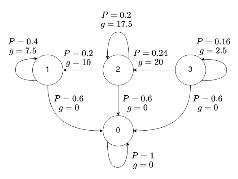
Auxiliary Stochastic Shortest Path : equivalent Discounted Problem

Dynamics : $$ \begin{aligned} p_{w|x,u}(j|i,u) &= \alpha \tilde P_{ij}(u) \ p_{w|x,u}(0|i,u) &= 1-\alpha \ p_{w|x,u}(j|0,u) &= 1 \ p_{w|x,u}(0|0,u) &= 1 \end{aligned} $$

Cost :

$g(x_k,u_k,w_k) = \alpha^{-1}\tilde g(x_k,u_k,w_k)$

one to one mapping to discounted problem
Example : given discount factor $\alpha=0.4$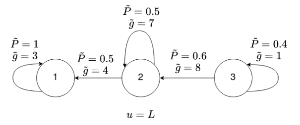

[SP]Shortest Path Problem

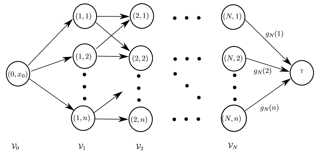
[DFS] Deterministic Finite State Problem : $$ x_{k+1} = f_k(x_k,u_k)\ J=g_N(x_N) + \sum_{k=0}^{N-1}g_k(x_k,u_k) $$ [SP] Shortest Path : in a graph, find a path from node $s\in \mathcal V$ to $t\in \mathcal V$ that has a smallest length $$ Q^* = \underset{Q\in\mathbb Q_{s,t}}{\text{argmin}} = \underset{Q\in\mathbb Q_{s,t}}{\text{argmin}}\sum_{h=1}^{q-1}c_{i_h,i_{h+1}} $$

symmetric : forward DPA and backward DPA are the same for this problem
no negative cycles : $\forall i\in\mathcal V, Q\in \mathcal Q_{i,i},J_Q\ge 0$ , if negative, there will exist infinite loop
$N\le|\mathcal V|-1$
DFS to SP
why it can be solved by forward DPA ($J_k\gets J_{k+1}$)? it's deterministic
why it can be solved by backward DPA ($J_k\gets J_{k-1}$)? it can be converted to a deterministic DP problem.

[HMM]Hidden Markov Model :

measurement model : $z$ is measure in transition from $i$ to $j$

$$ M_{ij}(z) = p_{z|x,w}(z|i,j) $$

Viterbi Algorithm : Given measured sequence $Z_1=(z_1,\cdots,z_N)$, we want to find the most likely state trajectory $X_0=(x_0,\cdots,x_N)$ $$ \begin{aligned} &\underset{X_0}{\text{max}}~p(X_0, Z_1) = p(x_0)\prod_{k=1}^N P_{x_{k-1}x_k}M_{x_{k-1}x_k}(z_k) \ \Leftrightarrow &\underset{X_0}{\text{min}}\left(c_{s,(0,x_0)}+\sum_{k=1}^Nc_{(k-1,x_{k-1}),(k,x_k)}\right) \end{aligned} $$ where $$ \begin{aligned} c_{s,(0,x_0)} &= \begin{cases} -\text{ln}(p(x_0))&p(x_0)>0 \ \infin & p(x_0) = 0 \end{cases} \ c_{(k-1,x_{k-1}),(k,x_k)}&=\begin{cases} -\text{ln}(P_{x_{k-1}x_k}M_{x_{k-1}x_k}(z_k)) & P_{x_{k-1}x_k}M_{x_{k-1}x_k}(z_k)>0\ \infin & P_{x_{k-1}x_k}M_{x_{k-1}x_k}(z_k) = 0 \end{cases} \ c_{(N-1,x_{N-1})} &= 0 \end{aligned} $$

DPA can be applied to already solve for the most likely state trajectory up until now.
Future measurements can change the most likely trajectory for pasttime steps

[LCA]Label Correcting Algorithm

$s\to \text{OPEN}$, set $d_s=0,d_j=\infin~\forall j\in \mathcal V/{s}$
$\text{OPEN}\rightarrow{i}\cup\text{OPEN}$
$\forall j\in \mathcal N_i$ if $(d_i+c_{ij})<d_j $ and $(d_i+c_{ij})<d_{t}$, $d_j\gets d_i+c_{i,j}$, $j.\text{parent} \gets i$; if $j\neq t$ , $\text{OPEN}\gets\text{OPEN}\cup{j}$
$|\text{OPEN}| > 0$ goto 2

# step 0, s is the initial seed
open_set = [s]
d = np.fill([n], np.inf)
d[s] = 0 

while len(open_set) > 0:
	# step 1 visit node in open set
    i = open_set.pop()
    for j in i.children:
        # step2 update the distance of j
        # d[i]+c[i,j]+h[j] < dt -> A-star
        # h:positive lower bound get from node j to T
        if d[i]+c[i,j] < d[j] and (d[i]+c[i,j]) <dT:
            d[j] = d[i] + c[i,j]
            j.parent = i
            if not j is T:
                open_set.append(j)

Search Order :
- Breadth-first
- Depth-first
- Best-first: $d_i$ the smallest nearest first
Dijkstra's Algorithm : $d_i$ best-first
A$^\star$ : $d_i+h_i$ best-first, where $h_i=\underset{k\in\mathcal V/{j}}{\text{min}}c_{jk}$

[HJB]Hamilton-Jacobian-Bellman Equation

$$ 0 = \underset{u\in\mathcal U}{\text{min}}\left(g(\text x,u) + \frac{\partial J^(t,\text x)}{\partial t} + \frac{\partial J^(t,\text x)}{\partial \text x}f(\text x,\text u)\right) $$

where $J^*(T,\text x)=h(x)$

Pontryagin's Minimum Principle : $$ \begin{aligned} H(\text x, \text u,\text p) &= g(\text x, \text u)+ \text p^\top f(\text x,\text u) \ \dot p(t) &= -\left.\frac{\partial H(\text x, \text u, \text p)}{\partial \text x}\right|^\top_{\begin{matrix}x(t)\u(t)\p(t)\end{matrix}} \ p(T) &= \left.\frac{\partial h(\text x)}{\partial\text x}\right|^\top_{x(T)} \ u(t) &= \underset{\text u\in \mathcal U}{\text{argmin}}H(x(t),\text u,p(t)) \ \dot x(t) &= f(x(t),u(t)) \end{aligned} $$

necessary condition for optimal cost
Bang-Bang Control : $u\in {a,b}$
- Example : $\ddot x = u, a<0<b$ , normally $u=\begin{cases}b & t\in[0,t]\a&t\in[t,T]\end{cases}$
minimize total time $T$: $g(\text x,\text u) = 1$, since $T=\int_0^T 1\text d\tau$

optimal trajectory $$ H(x(t),u(t),p(t)) = -\left.\frac{\partial J(t,x)}{\partial t}\right|_{x(t)} = \text{constant} $$