[ICP]Introduction to Computational Physics

Professor: Andreas Adelmann

1. Random Number Generator

Congruential RNG

$$ x_i = (cx_{i-1})mod~p $$

maximal period is $p-1$, maximal period reach if $c^{p-1}mod~p = 1$

Lagged Fibonacci RNG

$$ x_{b+1} = (\sum_{j\in\mathcal J}x_{b+1-j}) mod ~ 2\\ j\subset{1,\cdots, b} $$

initial sequence at least $c$ bits
usually use congruential RNG to obtain seed sequence

When $|j| = 2$ $$ x_{i+1} = (x_{i-c}+x_{i-d}) mod ~ 2 \ c,d\in{1,\cdots, i-1} $$ max period: $2^c - 1$

Zierler-Trinomial condition

$1+z^c+z^d$ cannot be factorized by in subpolynomials, smallest $(c,d) = (250,103)$

Square/Cubic Test

square test:$(s_i, s_{i+1})$
cubic test: $(s_i, s_{i+1}, s_{i+2})$

$\chi^2$ test

fluctuation of mean value, mean value should be gaussian $$ \chi^2 = \sum_{i=1}^k\frac{N_i-\frac{n}{k}}{\frac{n}{k}} $$

$n$ : number of samples

$N_i$ : count number for each bin

$k$ : number of bins

Monte Carlo

expected error for MC sampling is $\mathcal O(\frac{1}{\sqrt N})$

error bound in quasi-MC is $\mathcal O(\frac{(log~N)^d}{N})$

D-star Discrepency

$$ D^*N = \underset{0\le v_j \le 1}{max}\left|\frac{1}{N}\sum{i=1}^N\prod_{j=1}^d1_{0\le x_j^i \le v_j} - \prod_{j=1}^dv_j\right| $$

it measure how dense the points distributed inside a given volume

$N$ : number of dataset points ${x^1,\cdots,x^n}$

$d$ : dimension of the points

low-discrepancy : $D^*_N \le c(d)\frac{log(N)^d}{N}$

Uniform Sphere Shell

given uniform distribution $X,Y\sim Unif(0,1)$, get 3d sphere uniform distribution

$$ \int_0^X\int_0^Y dxdy = \int_0^\Phi\int_0^\Theta \frac{1}{4\pi} sin\theta d\phi d\theta \\ \Rightarrow XY = \frac{1}{4\pi}(1-cos\Theta)\Phi $$ let $\Phi = 2\pi X$ then $\Theta = acos(1-2Y)$

$\therefore S\sim [Rsin\Theta cos\Phi, Rsin\Theta sin\Phi, Rcos\Theta]$

Uniform Ellipse

rejection sampling, sample $X\sim Unif(-a, a), Y\sim Unif(-b,b)$, accept the points inside ellipse
draw $X,Y\sim Unif(0,1)$, $\psi = atan(\frac{b}{a}tan(2\pi X))$, $r = \sqrt Y \frac{ab}{\sqrt{(b cos\psi)^2 + (a\sin\psi)^2}}$, $E\sim [rcos\psi, rsin\psi]$

Uniform to Gaussian

$$ y_1 = \sqrt{-\sigmaln(1-z_2)}sin(2\pi z_1)\\ y_2 = \sqrt{-\sigmaln(1-z_2)}cos(2\pi z_1) $$

using uniform $z_1$ and $z_2$ could get two gaussian $y_1$ and $y_2$

2. Percolation

cirtical point $p_c$: occupation probabilty $p$, a phase transition from non-percolated system to percolated system containing an infinitely-sized cluster
percolation strength $\beta$: $P(p\gtrsim p_c) \sim |p-p_c|^\beta$, how fast the transition
wrapping probability : $W(p) = \begin{cases}0 & 0\leq p<p_c \ 1 & p_c< p\le 1\end{cases}$
cluster-size distribution: $n_s(p)=\underset{L\rightarrow \infin}{lim}\frac{N_s(p,L)}{L}$, $N_s(p,L)$ is the number of cluster of size $s$ given occupation probability $p$ and system's side length $L$

Burning Method

def burning_method(lattice):
    """
    	lattice:	np.ndarray[L, L]
    				0 means empty, 1 means occupied
    """
    t = 2
    lattice[0, lattice[0, :] == 1] == t
    while True:
        t += 1
        has_changed = False
        for node in np.where(lattice == t):
            for neighbor in get_neighbors(node):
                if lattice[neighbor] == 1:
                    lattice[neighbor] = t
        		    has_changed      = True 
        at_bottom = (node[0] == lattice.shape[0] - 1).any()
        if not has_changed or at_bottom:
            break

Hoshen-Kopelman Algorithm

compute how many clusters

def hoshen_kopelman_algorithm(lattice):
    """
    	lattice:	np.ndarray[L, L]
    				0 means empty, 1 means occupied
    """
    cluster_sizes = [None, None] # starts with 2
    k = 2
    for i in range(lattice.shape[0]):
        for  j in range(lattice.shape[1]):
            if is_top_and_left_empty(lattice[i, j]): # new cluster
                lattice[i, j] = k
                cluster_sizes.append(1)
                k += 1
            else is_top_left_same_cluster(lattice[i, j]): # one neighbor in cluster or neighbors in same cluster
                lattice[i, j] = get_top_left_cluster(lattice[i,j])
                cluster_sizes[lattice[i, j]] += 1
            else: # neighbors in different cluster
                k1, k2 = get_top_left_cluster(lattice[i, j])
                lattice[i, j] = k1
                cluster_sizes[k1] += cluster_sizes[k2]
                mark_cluster_size_as_transferred(cluster_sizes, k2)

3. Fractals

fractal dimension $d_f$: stretch the object by $a$, the volume grows $a^{d_f}$ $$ \frac{V_\varepsilon^*}{\varepsilon^d} = \left(\frac{L}{\varepsilon}\right)^{d_f} $$
correlation function $c(r)$ : number of filled sites with in sphere $r$ shell $\Delta r$ normalized by surface
$$ c(r) \propto \begin{cases} C + exp(-\frac{r}{\xi}) & p<p_c\ r^{-(d-2 + \eta)} & p\approx p_c \end{cases} $$ $\xi$ is the correlation length $$ \xi \propto |p-p_c|^\nu~~where~~\nu=\begin{cases}\frac{4}{3}&2d \ 0.88 & 3d\end{cases} $$

$$ \eta = \begin{cases} \frac{5}{24} & 2d \ -0.05 & 3d\end{cases} $$

$$ d_f = d - \frac{\beta}{\nu} $$

$\beta$ : percolation strength

$d$ : dimension

Sandbox Method

def sandbox_method(lattice):
    """
    	lattice:	np.ndarray[L, L]
    				0 means empty, 1 means occupied
    """
    R  = []
    N_R = []
    c = lattice.shape[0]/2 - 1 # as python starts from 0
    for r in range(1, int(L//2)): # increase the sanbox size over iteration
    	R.append(r)
    	N_R.append(sum(lattice[c-r:c+r, c-r:c+r]==1))
    plot_log(R, N_R) # the fractal dimension d_f is the slope

Box Counting Method

def box_counting_method(lattice):
    """
    	lattice:	np.ndarray[L, L]
    				0 means empty, 1 means occupied
    """
    epsilon_inv = []
    N_epsilon   = []
    for epsilon in range(1, lattice.shape[0]):
    	boxes = maxpool2d(lattice, kernel=np.ones([epsilon, epsilon]), padding=0) # use the pooling to compute box
    	N_epsilon.append(sum(boxes > 0))
        epsilon_inv.append(1 / epsilon)
    plot_log(epsilon_inv, N_epsilon) # the fractal dimension d_f is the slope

4. Cellular Automata

cellular automata:$(\mathcal L, \psi, R,\mathcal N)$

$\mathcal L$ : $d$ dimension lattice of cells

$\psi$ : $m$ dimension boolean state for each site at time $t$

$R$ : $m$ rules to update the $\psi$

neighborhoods

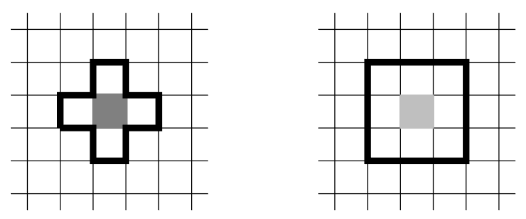
left:Von Neumann neighborhood : 4 (north-east-south-west)
right:Moore neighborhood : 8 (3x3 region)

boundary conditions

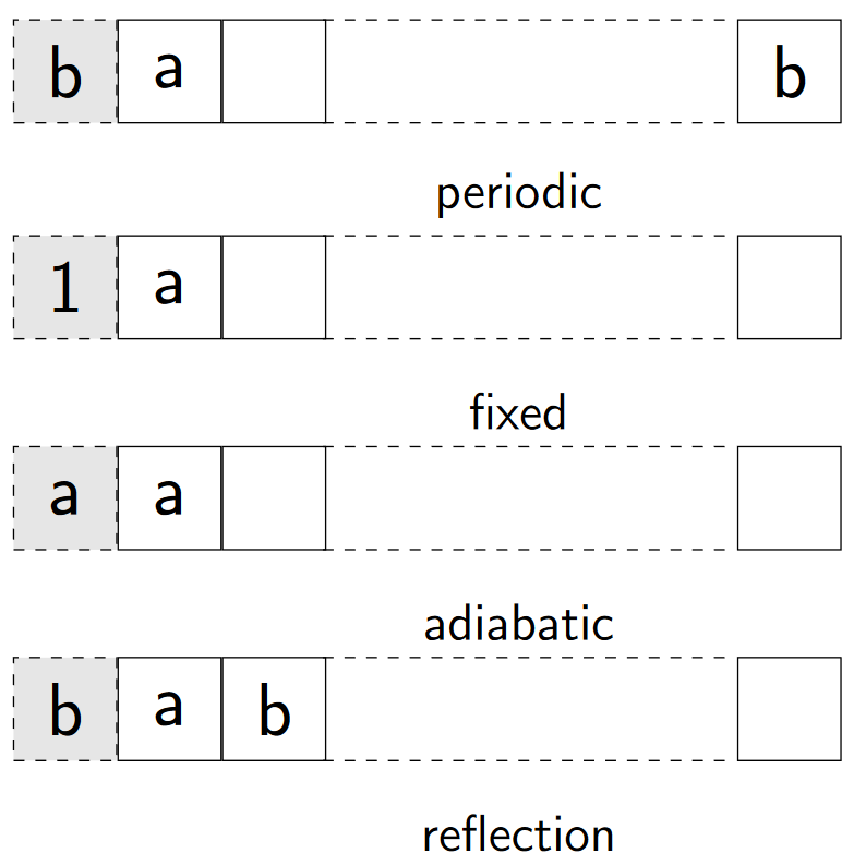
assume x[1:] is the actual space

periodic : x[0] = x[-1]
fixed : x[0] = C
adiabtic : x[0] = x[1]
reflection: x[0] = x[2]

Game of Life

moore neighborhood

$n < 2$ : 0 dead because of isolation
$n = 2$ : stay as before
$n = 3$ : 1 birth
$n>3$ : 0 dead because of over population

Langton Ant

enter white cell, turn left and paint cell gray
enter gray cell, turn right and paint cell white

observation

chaotic phase of about 10000 steps
formation highway
walking on highway

Traffic Models

$$ (\psi_{i-1},\psi_i,\psi_{i+1})_t \rightarrow (\psi_i)_{t+1} $$

rule \$(\psi_{i-1}\psi_{i}\psi_{i+1})_t$	111	110	101	100	011	010	001	000
184 $(\psi_{i})_t$	1	0	1	1	1	0	0	0

Gas of Particles ( HPP model )

$\psi(r, t) = (1011)$

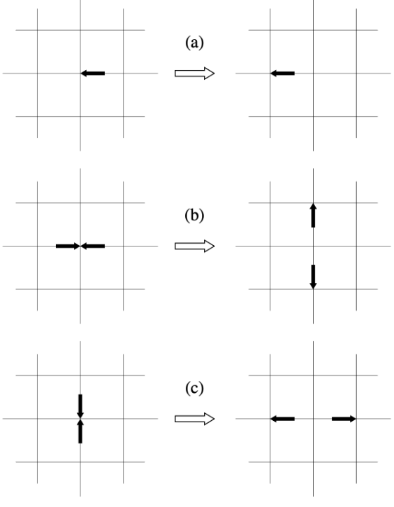
collision
propagation

5. Monte Carlo Method

Error

$$ \Delta \propto \frac{1}{\sqrt N} $$

$\boldsymbol \pi$ Buffon's Needle Experiment

$$ \pi(N) = 4\frac{N_c(N)}{N}\\ $$

$N_c$ : points in the quarter circle

Monte Carlo Integral

$$ \int_a^b g(x)dx \approx \frac{b-a}{N}\sum_{i=1}^N g(x_i) \equiv Q $$

$x_i$ is uniform sampled in $[a, b]$

$N$ is the number of samples

error $\propto (\Delta x)^2 \propto N^{-\frac{2}{d}}$

Center Limit Theorem $$ \delta Q = (b-a) \frac{\sigma}{\sqrt{N}} = V\frac{\sigma}{\sqrt{N}}\

\sigma^2 = \frac{1}{N-1}\sum_{i=1}^N \left(g(x_i) - \frac{Q}{N}\right) $$ $V$ : is the volume of hypercube for integration in high dimension

the error independent of dimension $d$

cirtical point $$ N^{-\frac{2}{d}}\overset{crit}{=}\frac{1}{\sqrt{N}} $$ for $d>4$, MC more efficient

high dimension integration

hard-sphere, overlap $\rightarrow$ rejective

Importance Sampling

$$ \int_a^b f(x)dx \approx \frac{1}{N}\sum_{i=1}^N \frac{f(x_i^G)}{g(x_i^G)} $$

$x_i^G$ is sampled according to distribution $g(x)$

$G(x)$ is the cdf of $g(x)$, $G(x) = \int_a^x g(x)dx$

$f$ and $g$ need to be positively correlated

Control Variates

$$ \int_a^b f(x)dx = \int_a^b (f(x)-g(x))dx + \int_a^b g(x)dx $$

$f$ and $g$ need to be positively coorelated

$Var(f-g) < Var(f)$
$\int_a^b g(x)dx$ is known

Quasi Monte Carlo

$$ D^*_N = \mathcal O\left(\frac{(log N)^d}{N}\right) $$

$$ \mathcal O(\frac{(logN)^d}{N}) < \mathcal O(\frac{1}{\sqrt{ N}}) \Rightarrow N > 2^d $$

Markov Chain

$$ \frac{dp(X,\tau)}{d\tau} = \sum_{Y\neq X} p(Y)W(Y\rightarrow X) - \sum_{Y\neq X} p(X)W(X\rightarrow Y)\\ W(X\rightarrow Y) = T(X\rightarrow Y) A(X\rightarrow Y) $$

$A(X\rightarrow Y)$ means the accpet probability from $X$ to $Y$

$T(X\rightarrow Y)$ means the transition probablity from $X$ to $Y$

ergodicity: $\forall X,Y: W(X\rightarrow Y) > 0 $
normalization: $\sum_Y W(X\rightarrow Y) = 1$
homogeneity: $\sum_Y p(Y)W(Y\rightarrow X) = p(X)$

Detailed Balance : $\frac{d~p(X,\tau)}{d\tau} = 0$

M(RT)^2^ Algorithm

random choose a configuration $X$
compute $\Delta E = E(Y) - E(X)$
spinflip if $\Delta E < 0$ else accept iwth probability $exp(-\frac{\Delta E}{k_BT})$

Ising Model

simulate the magnetic properties of a material $$ \mathcal H = - J \sum_{i,j}S_iS_j - H\sum_i S_i $$ $S_i$ means the spin at position $i$

$j$ : is the neighbor off $i$

def ising_model(lattice, M, E, J, beta, steps):
    """
    	lattice:	np.ndarray[L, L]
    				1 means spin up, -1 means spin down
    	M:			float
    				magnetic field
    	E:			float 
    				energy
    	J:			float
    				coupling constant
    	beta:		float
    				inverse of temperature `beta = 1 / T / kB`
    	steps:		int
    """
    L = lattice.shape[0]
    for i in range(steps):
        x, y = np.random.randint(0, L, [2])
        sigma_j = lattice[get_neighbors(lattice, x, y)].sum()
        sigma_i = lattice[x, y]
        delta_E = 2 * J * sigma_i * sigma_j
        accept = min(1., exp(-beta * delta_E)) > rand()
        if accpet:
        	M -= 2*lattice[x, y]
            E += delta_E
            lattice[x, y] *= -1
   return M, E

random choose a configuration $X$
compute $\Delta E = E(Y) - E(X) = 2J\sigma_i\sigma_j$
spinflip if $\Delta E < 0$ else accept with probability $exp(-\frac{\Delta E}{k_BT})$

Multilevel Monte Carlo(MLMC)

$$ \mathbb E[P_L ] = \mathbb E[P_0] + \sum_{l=1}^L \mathbb E [P_l - P_{l-1}] $$

$$ N_l = \mu \sqrt{\frac{V_l}{C_l}}\\ C = \sum_{l=1}^L C_l N_l \\ Var = \sum_{l=1}^L V_l N^{-1}_l $$

$C_l$ : cost at level $l$

$V_l$ : variance at level $l$

$N_l$ : sample number at level $l$

6. Finite Difference

Error

input data error
rounding error
truncation error
simplification in mathematical model
human & machine error

propogation $$ \varepsilon \approx \sqrt{\sum_{i}^n \left(\frac{\partial f}{\partial x_i}\right)^2\varepsilon_i^2} $$

Partial Differential Equation (PDE)

parabolic : $D\frac{\partial ^2 \phi}{\partial ^ 2 x} - \frac{\partial \phi}{\partial t} = 0$
hyperbolic : $\frac{\partial^2 \phi}{\partial ^2 x} - \frac{1}{c}\frac{\partial^2 \phi}{\partial^2 t} = 0$

generate solution is $\phi(x,t)=\alpha f_0(x-ct)+\beta g_0(x+ct)$
elliptic : $\nabla^2\phi = 0$

Lagrange Derivative : $$ \frac{D\phi}{Dt} = \frac{\partial \phi}{\partial t} + \overrightarrow u \cdot \nabla \phi $$

Forward in Time, Backward in Space (FTBS)

$$ \begin{aligned} \frac{\partial \phi^{n+1}j}{\partial t} &= \frac{\phi_j^{n+1} - \phi_j^{n}}{\Delta t } + \mathcal O(\Delta t ) \ \frac{\partial \phi^n_j}{\partial x} &= \frac{\phi_j^{n} - \phi{j-1}^{n}}{\Delta x} + \mathcal O(\Delta x) \end{aligned} $$

first order accurate

explicit

Centred in Time, Centred in Space (CTCS)

$$ \begin{aligned} \frac{\partial \phi_j^n}{\partial t } &= \frac{\phi_j^{(n+1)}-\phi_j^{(n-1)}}{2\Delta t} + \mathcal O(\Delta t^2)\\ \frac{\partial \phi_j^n}{\partial x} &= \frac{\phi_{j+1}^n - \phi_{j-1}^n}{2\Delta x} + \mathcal O(\Delta x^2) \end{aligned} $$

second order accurate

implicit

Backward in Time, Centred in Space (BTCS)

$$ \frac{\partial \phi_j^n}{\partial t} = \frac{\phi_j^{n+1}-\phi_j^n}{\Delta t}+ \mathcal O(\Delta t)\\ \frac{\partial \phi_j^n}{\partial x} = \frac{\phi_{j+1}^n - \phi_{j-1}^n}{\Delta x } + \mathcal O(\Delta x)\\ $$

first order accurate

implicit

Stability

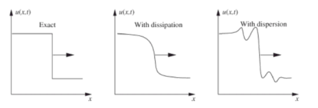
Dissipation : smooth out sharp corners, gradients, discontinuities
Dispersion : dependence of wave speed on wavelength

Lax-Equivalence Theorem

consistency + stability $\Leftrightarrow$ convergence

Courant-Friedrichs-Lewy(CFL) cirterion $$ C = \frac{u\Delta t}{\Delta x} \le C_{max} $$ for explicit, $C_{max} = 1$, much larger for implicit, as it's much more stable

Domain of Dependence(DoD)

DoD for FTBS $0\le c \le 1$
DoD for CTCS $-1 \le c \le 1$

Von-Neumann Stability Analysis $$ \phi^{n+1} = A\phi^n $$

$|A|^2 < 1$ stable and damping
$|A|^2 = 1$ neutral stable
$|A|^2 > 1$ unstable and amplyfying

for FTBS $$ \begin{aligned} \phi^{n+1}j &= \phi^n_j - c(\phi^n_j -\phi^n{j-1}) \ A^{n+1} e^{ikj\Delta x} &= A^n e^{ekj\Delta x} - cA^n\left(e^{ikj\Delta x}-e^{ik(j-1)\Delta x}\right) \ A &= 1 - c(1-e^{-ik\Delta x}) \ |A|^2 &= 1 - 2c(1-c)(1-cos k \Delta x) \end{aligned} $$ $c = \frac{u\Delta t}{\Delta x}$

if $u < 0 $ or $\frac{u\Delta t}{\Delta x} > 1$ the FTBS is unstable , which is $0\le c\le 1$

for FTCS $$ |A|^2 = 1 + 4c^2 sin^2(k\Delta x) $$ for CTCS $$ \begin{aligned} \phi_j^{n+1} &= \phi_j^{n-1}- c(\phi_{j+1}^n - \phi_{j-1}^n) \ A & = -ic sin(k\Delta x)\pm \sqrt{1 - c^2 sin^2 k\Delta x}\ |A|^2 &= 2c^2sin^2(k\Delta x) - 1 \mp sin(k\Delta x)\sqrt{c^2sin^2(k\Delta x) - 1} \end{aligned} $$

$|c| > 1$ unstable
$|c| \le 1$ stable

there are two solutions ,should ignore the spurious solution

Conservation

$$ \begin{aligned} M^{n+1} &= \int_0^1 \phi^{n+1}_x dx \\ = M^{n} &= \int_0^1 \phi^n_xdx \end{aligned} $$

Phase Velocity

$$ \phi(x,t )= \phi(x-ut,0) $$

$u$: phase speed

for CTCS, small $k$ and $\Delta x$ is correct

Shallow Water Equation

$$ H = H_0 + \eta $$

where $H$ is the water height, $\eta$ is the fluctuation $$ \frac{\partial u}{\partial t} + (u \cdot \nabla)u = -\frac{1}{\rho}\nabla p + g\ \nabla \cdot u = 0 $$

$$ \frac{\partial u_i}{\partial t} + u_j\frac{\partial u_i}{\partial x_j} = -\frac{1}{\rho} \frac{\partial p}{\partial x_i} + g_i \\ \frac{\partial u_i}{\partial x_i} = 0 $$

where $g = [0, 0, g_z]$ is the velocity

A-Grid(unstaggered) $$ \frac{\eta^n_j - \eta^{n-1}j}{\Delta t} = - H_0 \frac{u^n{j+1} - u^n_{j-1}}{\Delta x} \ \frac{u^{n+1}j - u^n_j}{\Delta t} = -g \frac{\eta^n{j+1} - \eta^n_{j-1}}{\Delta x} $$ courant number $c = \sqrt{gH_0}\frac{\Delta t}{\Delta x}$

stable for $c\le 2$

**C-Grid(Staggered) ** $$ \frac{\eta_j^n- \eta^{n-1}j}{\Delta t} = - H_0\frac{u^n{j+\frac{1}{2}}-u^n_{j-1}}{\Delta x} \ \frac{u^{n+1}{j+\frac{1}{2}} - u^n{j+\frac{1}{2}}}{\Delta t} = - g \frac{\eta^n_{j+1} - \eta^n_{j-1}}{\Delta x} $$ stable for $c\le 1$

7. Time Integration

error

truncation error : taylor expansion in euler method, $\mathcal O(\Delta t^2)$ for each step, $\mathcal O(\Delta t)$ in total
round-off error : charcteristic number $\eta$ , the smallest incremental, in euler method $\mathcal O(\eta)$ for each step, $\mathcal O(\frac{\eta}{\Delta t})$ in total
total error : for euler method, $\varepsilon \sim \frac{\eta}{\Delta t} + \Delta t$

one step method

for ordinary differential equatiion (ODE) $$ \frac{\partial \phi}{\partial t} = f(t, \phi(t))\quad \phi(t_0) = \phi^0 $$

$$ \frac{\phi^{n+1}-\phi ^n}{\Delta t} = \gamma f(t+\Delta t, \phi^{n+1}) + (1-\gamma)f(t,\phi^n) $$

multi step method

$$ \frac{(1+\beta)\phi^{n+1}-(1+2\beta)\phi^n + \beta\phi^{n-1}}{\Delta t} = \gamma f(t+\Delta t, \phi^{n+1}) + (1-\gamma + \alpha) f(t, \phi^n) - \alpha f(t-\Delta t, \phi^{n-1}) $$

name	$\beta$	$\gamma$	order
explicit euler	0	0	1
implicit euer	0	1	1
leapfrog	$-\frac{1}{2}$	0	2

Runge-Kutta method

$$ \begin{aligned} k_1 &= \Delta tf(t_n, \phi^n) \\ k_2 &= \Delta t f(t_{n+\frac{1}{2}}, \phi^n+\frac{k_1}{2})\\ k_3 &= \Delta t f(t_{n+\frac{1}{2}}, \phi^n+\frac{k_2}{2})\\ k_4 &= \Delta t f(t_{n+1}, \phi^n+k_3)\\ \phi^{n+1} &= \phi^n + \frac{k_1}{6} + \frac{k_2}{3} + \frac{k_3}{3} + \frac{k_4}{6} + \mathcal O(\Delta t^5) \end{aligned} $$

truncation error $\mathcal O(\Delta t^4)$

round-off error $\mathcal O(\frac{\eta}{\Delta t})$

minimum error is smaller with bigger $\Delta t$ compared to euler

Conservation

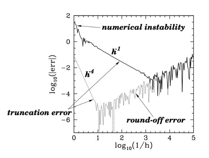
volume $\leftrightarrow$ energy

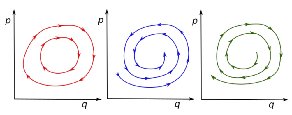
left: conserve
middle: loss energy
right: gain energy

Symplectic

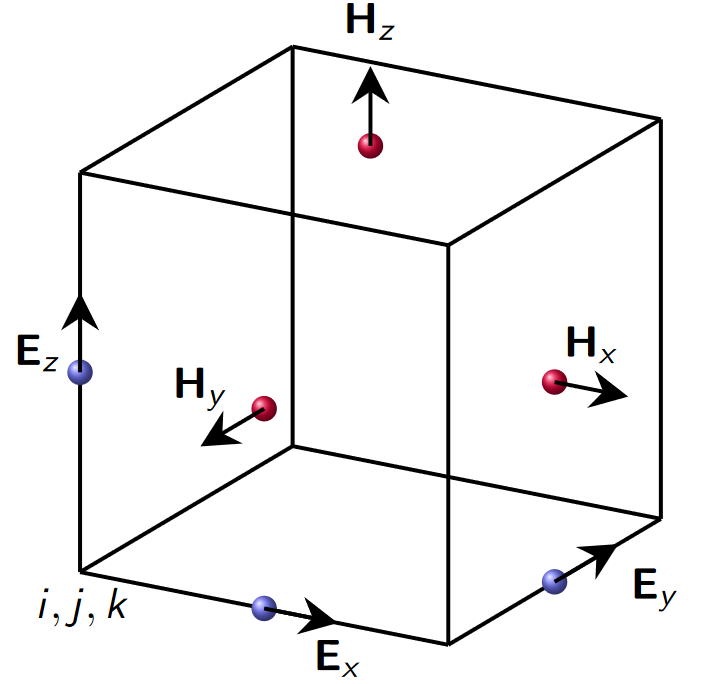
for Hamiltonian $[p, q]$ and $p = \dot q$ $$ \left[\begin{matrix} q(\tau)\ p(\tau) \end{matrix}\right] = A \left[\begin{matrix} q(0)\ p(0) \end{matrix}\right] $$ for energy conservation $|A| = 1$

8. Maxwell Equation

Valsov-Maxwell-Bolzmann equation

computational plasma $$ \begin{aligned} \frac{\partial f_s}{\partial t} + \nabla_x \cdot(\boldsymbol vf_s) + \nabla_{\boldsymbol v}\cdot ((\boldsymbol E + \boldsymbol v \times \boldsymbol B)\frac{q_sf_s}{m_s}) &= (\frac{\partial f_s}{\partial t})c \ \nabla \cdot \boldsymbol E &= \frac{\rho}{\varepsilon_0}\ \nabla \cdot \boldsymbol H &= 0 \ \nabla \times \boldsymbol E + \frac{\partial \boldsymbol H}{\partial t} &= 0\ \nabla \times \boldsymbol H - \mu_0 \varepsilon_0 \frac{\partial \boldsymbol E}{\partial t} &= \mu_0\sum_s q_s \int{-\infin}^{\infin} \boldsymbol vf_s d\boldsymbol v^3 \end{aligned} $$ where $f(x, \boldsymbol v, t)\in \mathbb R^{3\times 3\times}$ is the distribution $$ \begin{aligned} \boldsymbol D &= \varepsilon_0\varepsilon_r \boldsymbol E\ \boldsymbol B &= \mu_0 \mu_r \boldsymbol H \end{aligned} $$

Particle In Cell Method (PIC)

$$ \begin{aligned} \frac{d\boldsymbol x}{dt} &= \boldsymbol v\\ \frac{d\boldsymbol v}{dt} &= \frac{q}{m}(\boldsymbol E(\boldsymbol x,t), \boldsymbol v\times \boldsymbol B(\boldsymbol x, t)) \end{aligned} $$

Boris algorithm $$ \begin{aligned} \boldsymbol v^- &= \boldsymbol v^{n-\frac{1}{2}} + \frac{q}{m} \boldsymbol E^n\frac{\Delta t}{2} \ \frac{\boldsymbol v^+ - \boldsymbol v^-}{\Delta t} &= \frac{q}{2m}(\boldsymbol v^+ + \boldsymbol v^-) \times \boldsymbol B^n\ \boldsymbol v^{n+\frac{1}{2}} &= \boldsymbol v^+ + \frac{q}{m}\boldsymbol E^n\frac{\Delta t}{2} \end{aligned} $$ without $\boldsymbol E$ $$ \begin{aligned} \boldsymbol t &\approx \frac{q\boldsymbol B \Delta t}{2m}\ \boldsymbol s &= \frac{2\boldsymbol t}{1 + |\boldsymbol t|^2}\ \boldsymbol v' &= \boldsymbol v^- + \boldsymbol v^- \times \boldsymbol t\ \boldsymbol v^+ &= \boldsymbol v^- + \boldsymbol v' \times \boldsymbol s \end{aligned} $$

Yee Cell

$$ \begin{aligned} \frac{\partial \boldsymbol H}{\partial t} & = -\frac{1}{\mu_0} \nabla \times \boldsymbol E\\ \frac{\partial \boldsymbol E}{\partial t} &= \frac{1}{\varepsilon_0} \nabla \times \boldsymbol H \end{aligned} $$

$$ \begin{aligned} \frac{\partial \boldsymbol H_x}{\partial t} &= \frac{-1}{\mu_0} \left(\frac{\partial \boldsymbol E_y}{\partial z} - \frac{\partial \boldsymbol E_z}{\partial y}\right) & \frac{\partial \boldsymbol E_x}{\partial t} &= \frac{1}{\varepsilon_0}\left(\frac{\partial \boldsymbol E_y}{\partial z} - \frac{\partial \boldsymbol E_z}{\partial y}\right) \\ \frac{\partial \boldsymbol H_y}{\partial t} &= \frac{-1}{\mu_0}\left(\frac{\partial \boldsymbol E_z}{\partial x} -\frac{\partial \boldsymbol E_x}{\partial z}\right) & \frac{\partial \boldsymbol E_y}{\partial t} &=\frac{1}{\varepsilon_0}\left(\frac{\partial \boldsymbol E_z}{\partial x} - \frac{\partial \boldsymbol E_x}{\partial z}\right) \\ \frac{\partial \boldsymbol H_z}{\partial t} &=\frac{-1}{\mu_0}\left(\frac{\partial \boldsymbol E_x}{\partial y} - \frac{\partial \boldsymbol E_y}{\partial x}\right) & \frac{\partial \boldsymbol E_z}{\partial t} & = \frac{1}{\varepsilon_0}\left(\frac{\partial \boldsymbol E_x}{\partial y}-\frac{\partial \boldsymbol E_y}{\partial x}\right) \end{aligned} $$

$$ \frac{E_{x_k}^{n+\frac{1}{2}}-E_{x_k}^{n-\frac{1}{2}}}{\Delta t} = -\frac{1}{\varepsilon_0}\frac{H_{y_{k+\frac{1}{2}}}^n - H_{y_{k-\frac{1}{2}}}^n}{\Delta z} \\ \frac{H_{y_{k+\frac{1}{2}}}^{n+1}-H_{y_{k+\frac{1}{2}}}^n}{\Delta t} = -\frac{1}{\mu_0}\frac{E_{x_{k+1}}^{n+\frac{1}{2}}-E_{x_k}^{n+\frac{1}{2}}}{\Delta z} $$

error minimized by $\tilde E_{x} = \sqrt{\frac{\varepsilon_0}{\mu_0}}E_x$

stability: $\frac{\Delta t}{\Delta x} = \frac{1}{\sqrt d c}$

9. N-Body Problems

Particle in Cell Method (PIC)

$$ -\Delta \phi = \rho\\ F = -\nabla \phi $$

$\rho$ is the mass density, $\phi$ is the potential field $$ \phi(x) = G(x,x') * \rho(x') $$

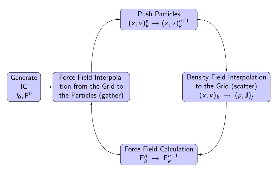
generate initial condition $f_0, F^0$
for loop
1. force field interpolate from grid to particles
2. push particles $(x,v)^n_k\rightarrow (x,v)^{n+1}_k$
3. density field interpolation to grid $(x,v)_k \rightarrow (\rho, J)_j$
4. force field calculation $F_k^n\rightarrow F_k^{n+1}$, using FFT
  
  $\phi(x) = \int \rho(x') G(x,x')dx' = \mathcal F^{-1}(\mathcal F(\rho) \cdot \mathcal F(G))$

Particle particle Particle Mesh(P3M)

$$ G(r) = \underbrace{\frac{1-erf(\alpha r)}{r}}{G{pp}} + \underbrace{\frac{erf(\alpha r)}{r}}{G{pm}} $$

$G_{pp}$ : use the n-body solver for short-range

$G_{pm}$ : use particle-mesh solver for long-range

walkerchi/ETHz-ICP

[ICP]Introduction to Computational Physics

1. Random Number Generator

Congruential RNG

Lagged Fibonacci RNG

Square/Cubic Test

$\chi^2$ test

Monte Carlo

D-star Discrepency

Uniform Sphere Shell

Uniform Ellipse

Uniform to Gaussian

2. Percolation

Burning Method

Hoshen-Kopelman Algorithm

3. Fractals

Sandbox Method

Box Counting Method

4. Cellular Automata

Game of Life

Langton Ant

Traffic Models

Gas of Particles ( HPP model )

5. Monte Carlo Method

Error

$\boldsymbol \pi$ Buffon's Needle Experiment

Monte Carlo Integral

Importance Sampling

Control Variates

Quasi Monte Carlo

Markov Chain

M(RT)^2^ Algorithm

Ising Model

Multilevel Monte Carlo(MLMC)

6. Finite Difference

Error

Partial Differential Equation (PDE)

Forward in Time, Backward in Space (FTBS)

Centred in Time, Centred in Space (CTCS)

Backward in Time, Centred in Space (BTCS)

Stability

Conservation

Phase Velocity

Shallow Water Equation

7. Time Integration

error

one step method

multi step method

Runge-Kutta method

Conservation

Symplectic

8. Maxwell Equation

Particle In Cell Method (PIC)

Yee Cell

9. N-Body Problems

Particle in Cell Method (PIC)

Particle particle Particle Mesh(P3M)