The goals / steps of this project are the following:
- Compute the camera calibration matrix and distortion coefficients given a set of chessboard images.
- Apply a distortion correction to raw images.
- Use color transforms, gradients, etc., to create a thresholded binary image.
- Apply a perspective transform to rectify binary image ("birds-eye view").
- Detect lane pixels and fit to find the lane boundary.
- Determine the curvature of the lane and vehicle position with respect to center.
- Warp the detected lane boundaries back onto the original image.
- Output visual display of the lane boundaries and numerical estimation of lane curvature and vehicle position.
1. Briefly state how you computed the camera matrix and distortion coefficients. Provide an example of a distortion corrected calibration image.
The codes for this step are contained in the 2nd and 3rd code cells of the IPython notebook located in "./adv_lane_detect.ipynb".
I start by preparing "object points", which will be the (x, y, z) coordinates of the chessboard corners in the world. Here I am assuming the chessboard is fixed on the (x, y) plane at z=0, such that the object points are the same for each calibration image. Thus, objp is just a replicated array of coordinates, and objpoints will be appended with a copy of it every time I successfully detect all chessboard corners in a test image. imgpoints will be appended with the (x, y) pixel position of each of the corners in the image plane with each successful chessboard detection.
I then used the output objpoints and imgpoints to compute the camera calibration and distortion coefficients using the cv2.calibrateCamera() function. I applied this distortion correction to the test image using the cv2.undistort() function and obtained the following results.
The camera calibration results are saved and used to undistort test images of road and lanes. cv2.undistort() function is called and the following result is captured.
The effect of camera calibration can be seen from the traffic sign of "Animal Crossing".
2. Describe how (and identify where in your code) you used color transforms, gradients or other methods to create a thresholded binary image. Provide an example of a binary image result.
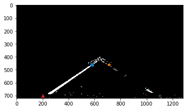
I used a combination of color and gradient thresholds to generate a binary image (the 6th to 12th code cells of the IPython notebook). A Gaussian noise kernel is used at first to blur the image. The thresholds of the x and y gradients, the overall gradient magnitude, the gradient direction, and the color threshold of the S channel are combined. An area of interest is applied to mask the image at last.
Here are examples of my output for this step.
3. Describe how (and identify where in your code) you performed a perspective transform and provide an example of a transformed image.
The code for my perspective transform includes a function called corners_unwarp(), which appears in the 16th code cell of the IPython notebook. Four points in a trapezoidal shape are picked up that would represent a rectangle when looking down on the road from above. The easiest way to do this is to investigate an image where the lane lines are straight, and find four points lying along the lines that, after perspective transform, make the lines look straight and vertical from a bird's eye view perspective. I chose the hardcode the source and destination points in the following manner:
area_of_interest = [[200,700],[150+430,460],[1150-440,460],[1100,700]]
src = np.float32(area_of_interest)

offset1 = 200 # offset for dst points x value
offset2 = 0 # offset for dst points bottom y value
offset3 = 0 # offset for dst points top y value
img_size = (img.shape[1], img.shape[0])
dst = np.float32([[offset1, img_size[1]-offset2], [offset1, offset3],
                      [img_size[0]-offset1, offset3],
                      [img_size[0]-offset1, img_size[1]-offset2]])
The source points are shown in the following straight lane image.
I verified that my perspective transform was working as expected by drawing the src and dst points onto a test image and its warped counterpart to verify that the lines appear parallel in the warped image.
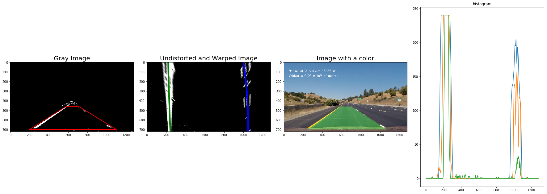
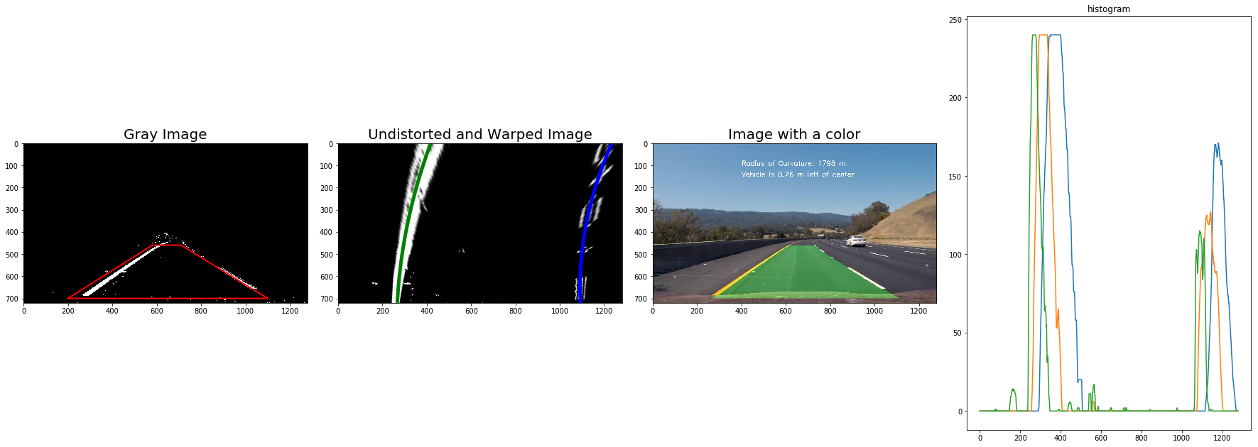
4. Describe how (and identify where in your code) you identified lane-line pixels and fit their positions with a polynomial? Describe how (and identify where in your code) you calculated the radius of curvature of the lane and the position of the vehicle with respect to center. Provide an example image of your result plotted back down onto the road such that the lane area is identified clearly.
Functions are defined to identify lane-line pixels: find_peaks(), find_lanes(), and fit_lanes().
Functions are defined to conduct sanity check for the lane and direction: sanity_check(), sanity_check_direction().
Functions are defined to compute the radius of curvature of the lane and the position of the vehicle with respect to center: find_curvature(), find_position().
The result of lane detection on a straight line test image is shown as follows:
The result of lane detection on a curve line test image is shown as follows:
Here's a link to my video result
Here's a link to my video result
Here's a link to my video result
1. Briefly discuss any problems / issues you faced in your implementation of this project. What could you do to make it more robust?
-
One issue I faced in this project is the use of the class
Line(), which keeps the characteristics of each line detection. One must be very clear about the inputs and outputs of each function and the method/logic of managing the tracks of lanes given previous detections and new detections. I referred to this Github repo to manage the tracks of lanes. -
The source and destination points in the perspective transformation are to be selected and tuned to accurately project the measurement back down onto the road.
-
After working out the given video in this project, I copied and tested the videos from Project 1 but received errors. The reason is that videos/images from Project 1 are in different size comparing to videos/images in this project --- they are cropped. I modified my functions to avoid hard-coded parameters, especially the shape of images. For videos from Project 1, the area of interest is redefined. Since (I guess) the videos are generated by the same camera but cropped, I tested the videos from Project 1 with and without camera calibration: there is no big difference between results with and without camera calibration.
Here's a link to my video result of straight lane without camera calibration
Here's a link to my video result of straight lane with camera calibration
- The current pipeline does not work on the
harder_challenge_video.mp4. The robustness of the pipeline should be enhanced, which can deal with sharp turns (e.g., U-turn). The area of interest should be tuned, the source and destination points in the perspective transformation should also be tuned. These are future works.
Here's a link to the result of pipeline failure on harder_challenge_video.mp4
- The computation of the radius of curvatures has been updated in the resubmission. The radius is measured in the middle of the polynomial rather than at the bottom of the image. The radius of curvatures are between 400-1500 meters for curves and values higher than 2500 m for when the road appears to be straight.


