University of Pennsylvania, CIS 565: GPU Programming and Architecture, Final Project
by Ashley Alexander-Lee, Matt Elser, and Wayne Wu.
Check it out live! (WebGPU Required)
- Clone this repo
- Run
npm i - Build with
npm run-script build - Start with
npm start - Must view using Google Chrome Canary or Chrome Developer
- Be sure to
--enable-unsafe-webgpuin the Chrome Settings
Camera Controls
Left Mouse Hold and Move: change camera orientationRight Mouse Hold and Move: pan cameraScroll in/out: zoom in/outresetCamera: gui control to reset camera to the scene's default
Grid Controls
gridWidth: change the number of divisions of the hash grid (hash grid size is constant)gridOn: turn the grid checkerboard visualization on or off
Scene Controls
scene: choose the scene configuration, which changes the number of agents, agent goals, camera default, and platform widthmodel: choose which model to useshowGoals: show where the agent goals are (marked with rainbow spheres)shadowOn: show the agent shadowsagent selector: choose the number of agents in powers of 2 (only supported in dense and sparse scenes)
Simulation Controls
simulate: start/stop simulationdeltaTime: the time step to use in the simulationlookAhead: parameter that affects how far the agents look ahead to plan their trajectoryavoidanceModel: use the avoidance model, which allows agents to move in a more tangential direction when stuck in a dense arearesetSimulation: reset the simulation
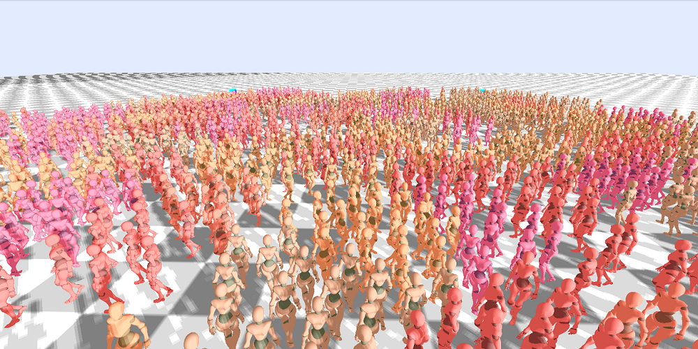
This project attempts to implement a real-time crowd simulation based on the paper: Position-Based Real-Time Simulation of Large Crowds. Unlike the paper which uses CUDA and Unreal Engine for simulation and rendering, this project uses WebGPU for both.
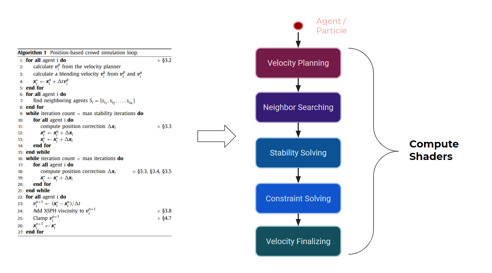
In WebGPU, we use compute shaders in replacement of CUDA kernels to simulate the agents. The algorithm can be broken down into five main processes including:
- Velocity Planning: advect the agent based on a calculated velocity field.
- Neighbor Searching: find the nearest neighbor and assign to hash grid.
- Stability Solving: resolve any collisions that remain from the previous time step for stability.
- Constraint Solving: project the main constraints and correct agents' positions.
- Velocity Finalizing: finalize the velocity and update the final position of the agent
In order to ensure our neighbor finding was efficient, we employed a hash grid neighbor finder, based on this article.
Each agent reacts to other agents within two radii: near radius and far radius. A naive solution to finding agents within these radii would be to iterate over all agents in the scene and check their distance. Instead, a hash grid is used. A uniform grid is (non-visually) overlayed onto the plane of agents. The following series of compute shaders turns this conceptual grid into a useful tool, entirely on the GPU:
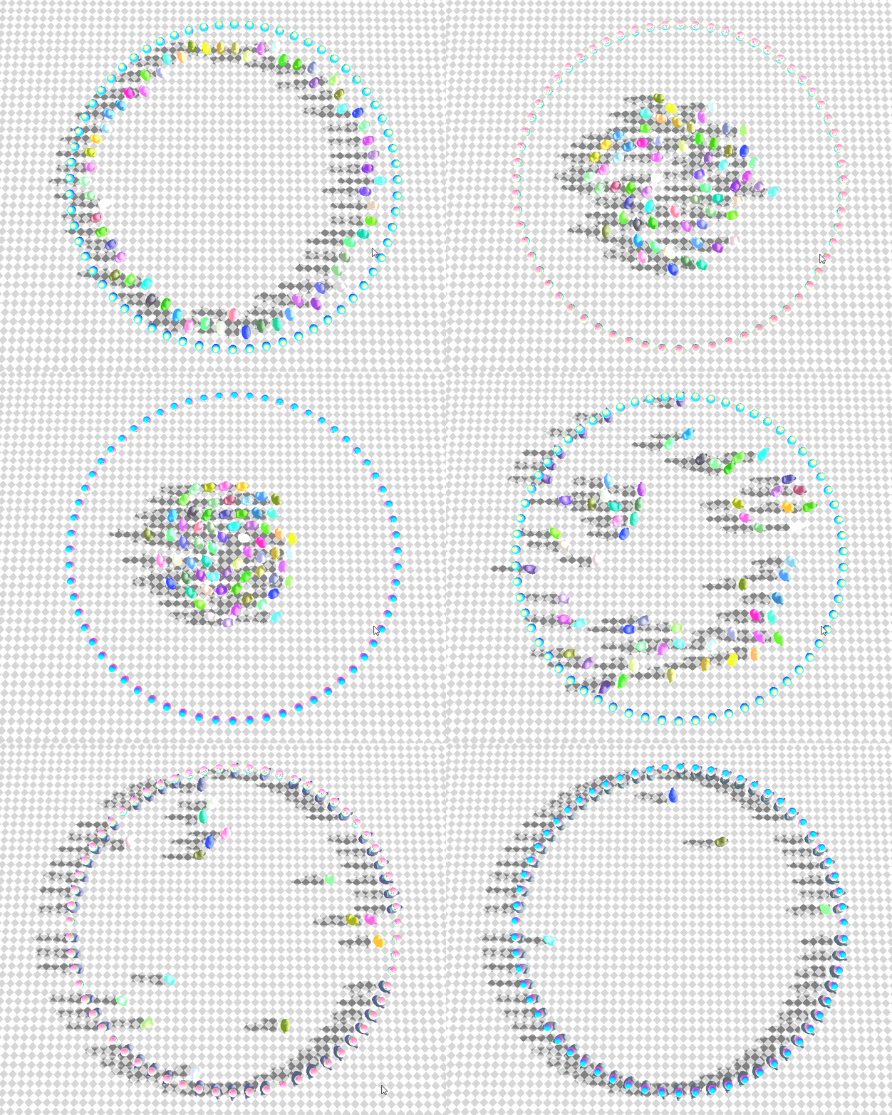
- For each agent, a thread on the GPU identifies the cell that agent belongs to. Agent's outside the finite hash grid are considered to be in an invalid cell and do not contribute to further computation/simulation, but are rendered grey for clarity.
- The agent buffer is then sorted based on these cells using a GPU based bitonic sort via a series of compute shaders. This is done in multiple shader calls as a device-wide join is needed after each step.
- Finally an additional compute shader determines where in the agent buffer each cell's agents starts and ends, storing that data in a cell buffer. For example, agents in cell 33 could occupy indicies X through Y, and agents in cell 34 could then be found at indicies Y+1 through Z. Having completed all this, all that is needed to find neighbors is to simply iterate over agents between the start and end for the relevant cells. The relevant cells in the paper's implementation are hardcoded to be 9 cells: the agent's current cell and all cells adjacent to it. Our implementation, however calculates which cells are within the relevant radius. This calculation not only makes our hash grid more efficient for larger/denser grids (by ignoring cells outside the agent's radius), it is more robust for smaller cell sizes where the agent's radius may reach farther than just the adjoining cells.
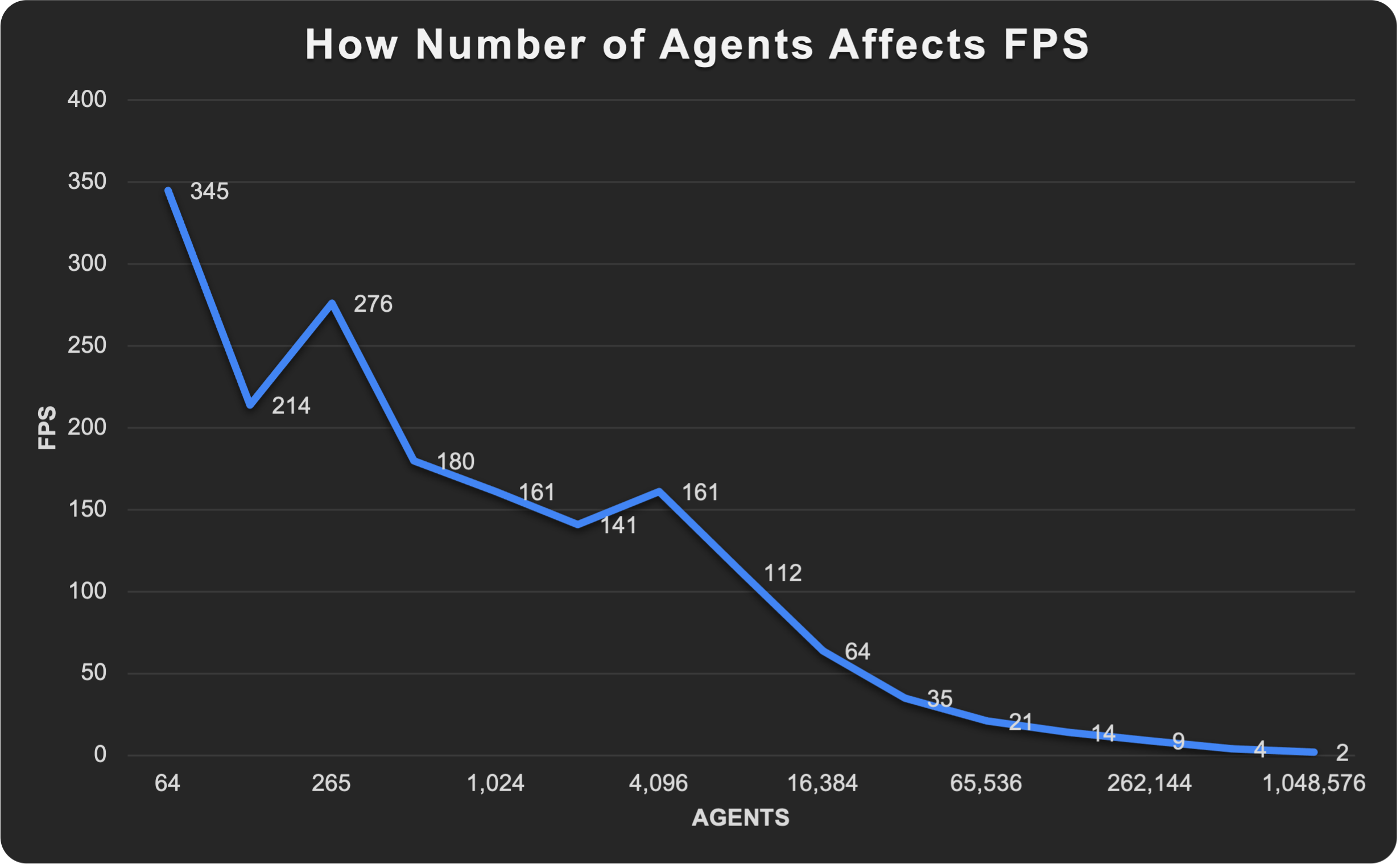
Our implementation can emulate a non-hashgrid implementation by setting the gridWidth parameter to 1 (to set the grid to be 1 cell wide by 1 cell long). By doing so the frame rate will notably drop in scenes with higher agent counts. Larger agent counts can be simulated more efficiently, reaching peak efficiency in the low hundreds with diminishing returns due to the overhead of calculating/referencing more cells for the same area of world-space. Notably, rearranging the agent buffer still allows for reading the agents contiguously in memory, which is the most efficient configuration for reads.
 Pictured above: A visualization of the early cell assignments, used to debug our initial implementation
The core algorithm of the paper is based on Position-based Dynamics with Jacobi Solver. Unlike the Gauss-Siedel method, the Jacobi solver can be more easily parallelized at the cost of slower convergence. While physically less accurate, PBD is really fast and therefore has been a popular simulation technique for real-time applications.
For more information on PBD, please refer to the original PBD paper.
The first constraint applied is a simple collision constraint model for short range collision. This resolves the immediate collisions between neighboring agents to prevent penetration.
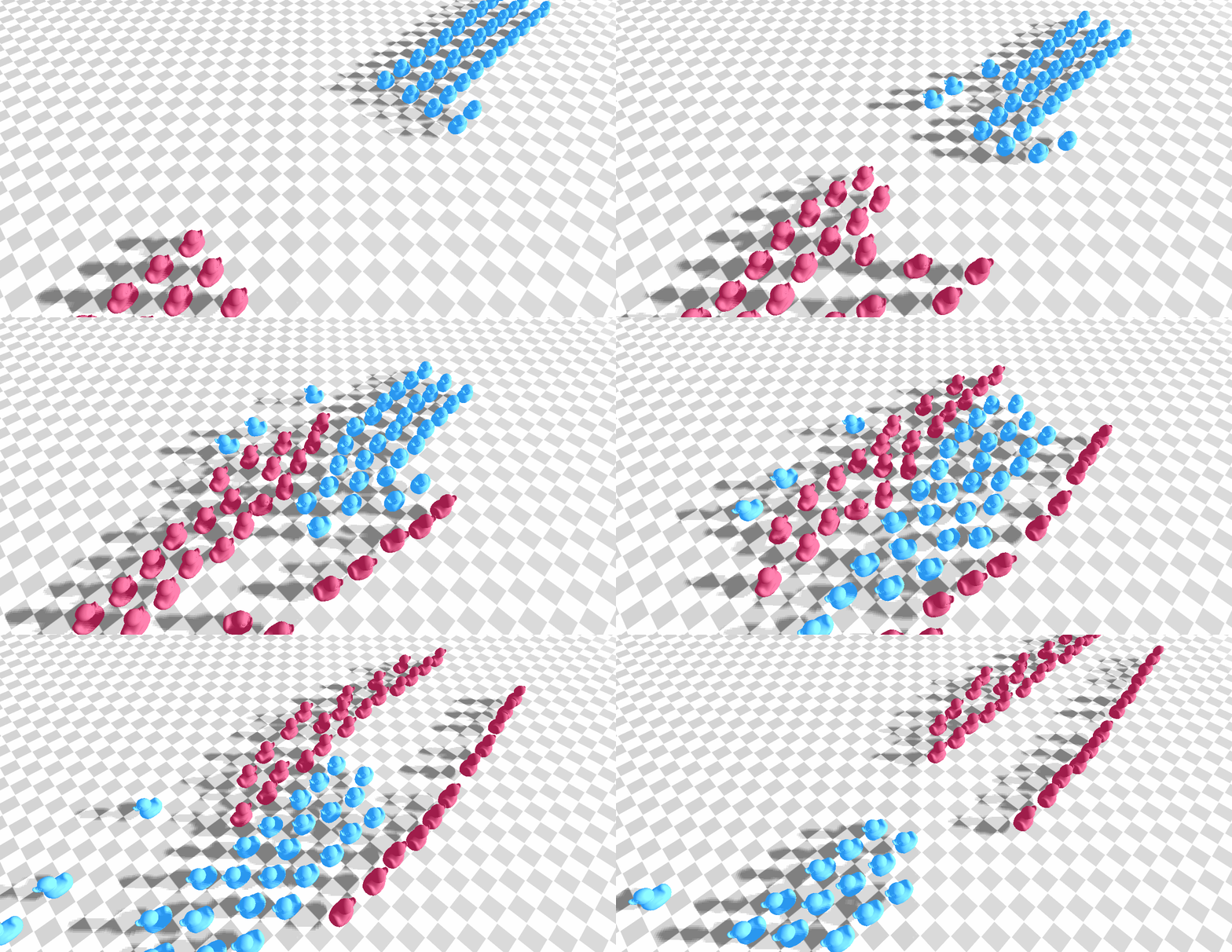
Long range collision constraint is used to enable agents to look ahead in the future for possible collisions. The constraint will predict the position of neighboring agents at a specified future time and resolve any collision at the future position. As shown in the image below, the agents start reacting before they are even close to colliding. User can tweak the lookAhead parameter to specify how far ahead to an agent should look ahead for long range collision.
| lookAhead = 6 | lookAhead = 12 |
|---|---|
 |
 |
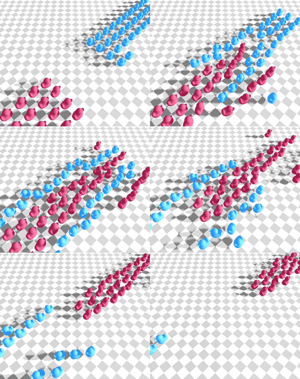
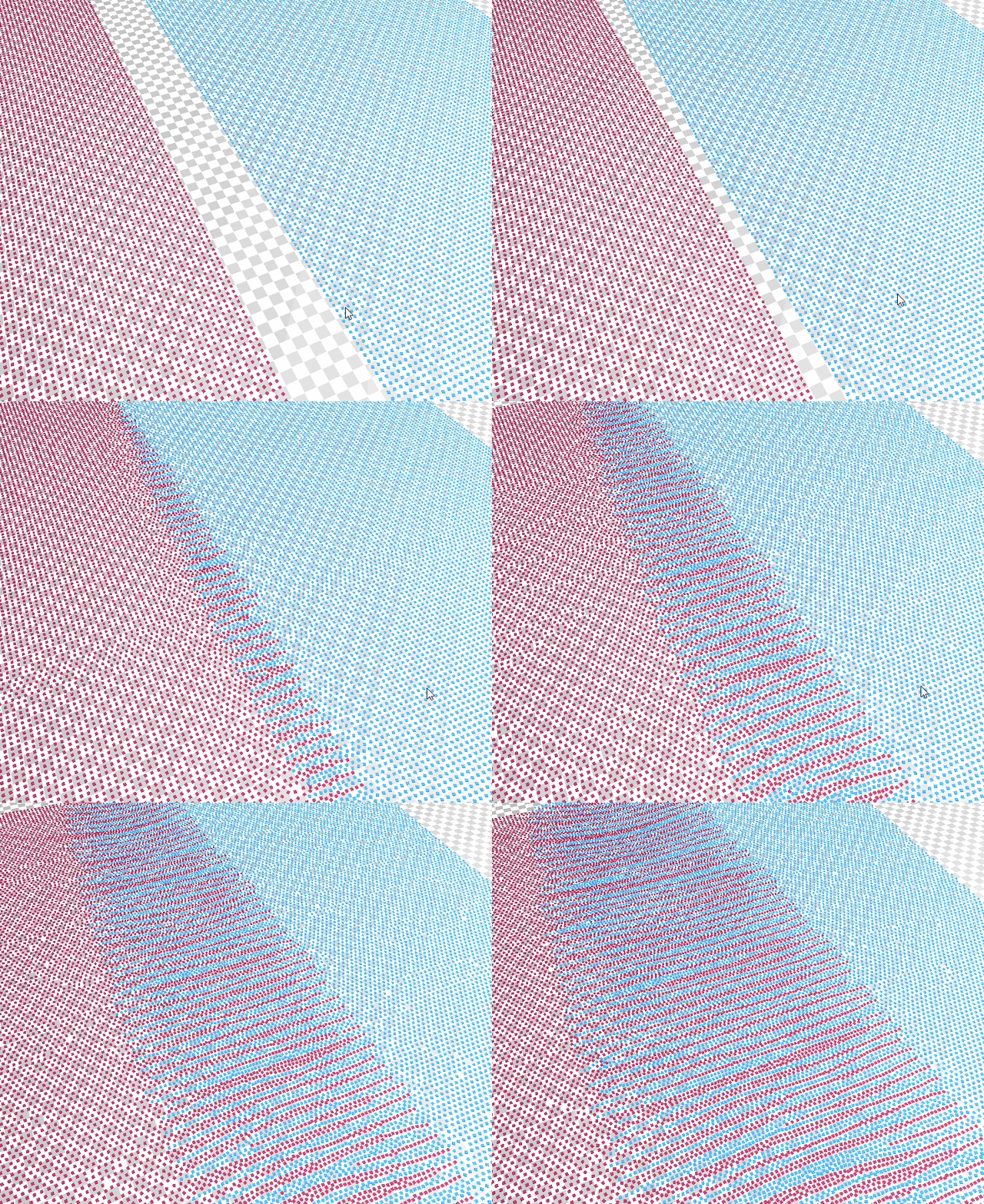
The paper introduces a novel addition to the long range collision constraint that prevents agents from being pushed back, typically in a dense crowd. The avoidance model considers only the tangential component of the position correction, thus removing/reducing the correction along the contact normal (which can push the agent back if two agents are walking towards each other).
| Scene | LR | LR w/ Avoidance |
|---|---|---|
| Proximal | 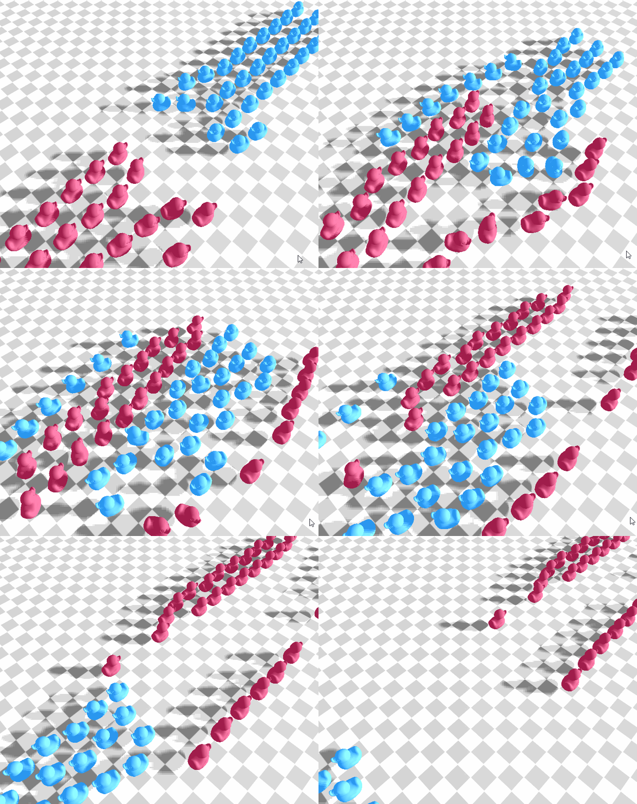 |
 |
| Dense | 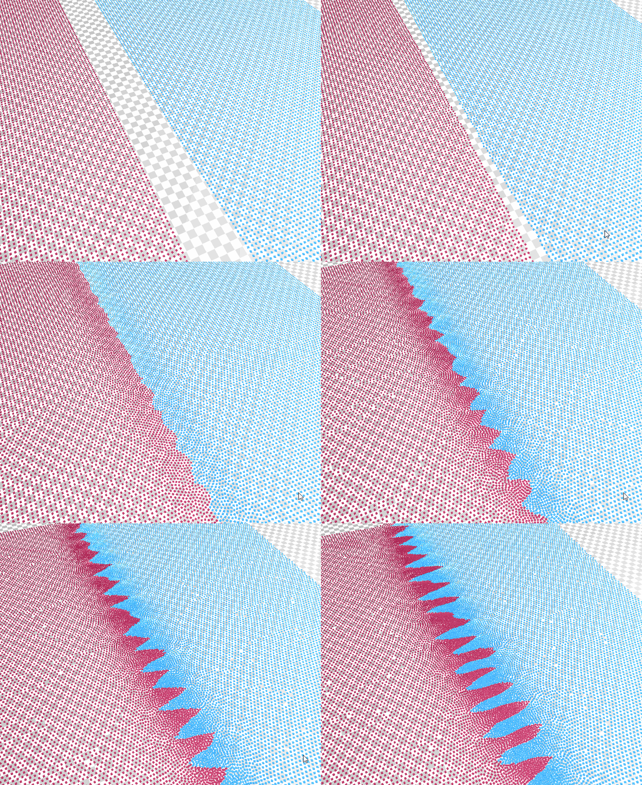 |
 |
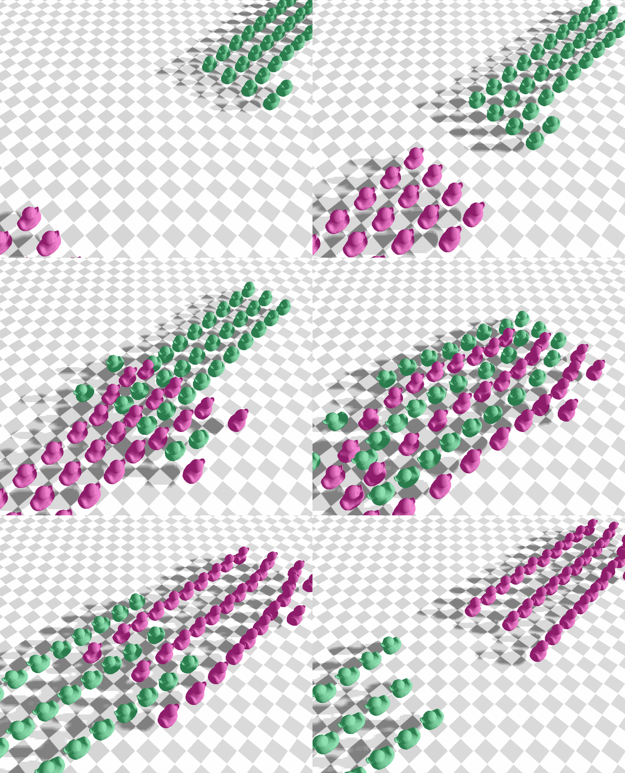
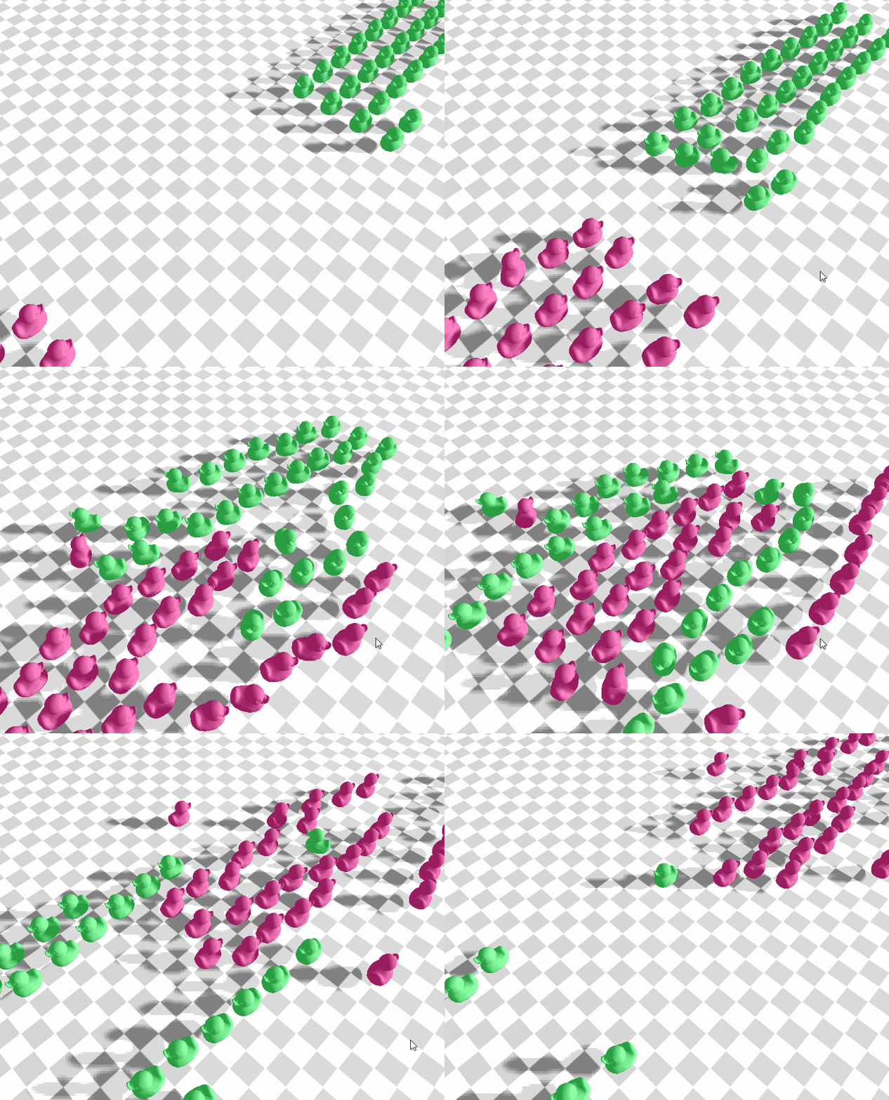
Cohesion is added so that agents within the same group will tend to follow each other thus creating smoother packed motions. When cohesion is off, it is more likely to see individual agents wander off alone as shown below.
| Debug | Cohesion OFF | Cohesion ON |
|---|---|---|
 |
 |
 |
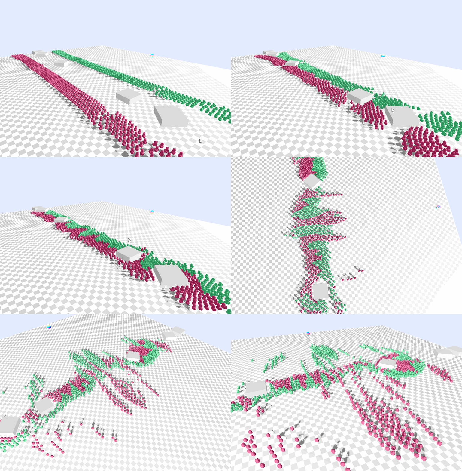
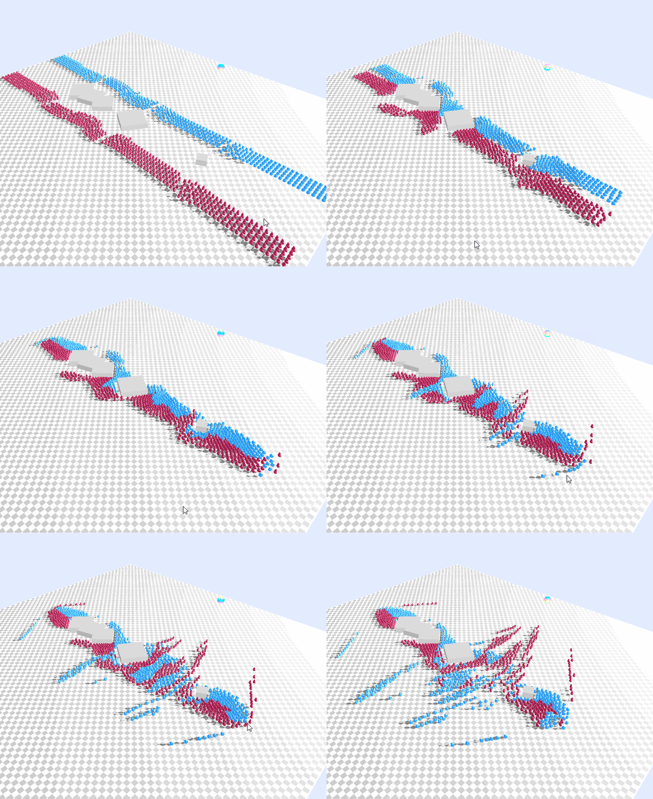
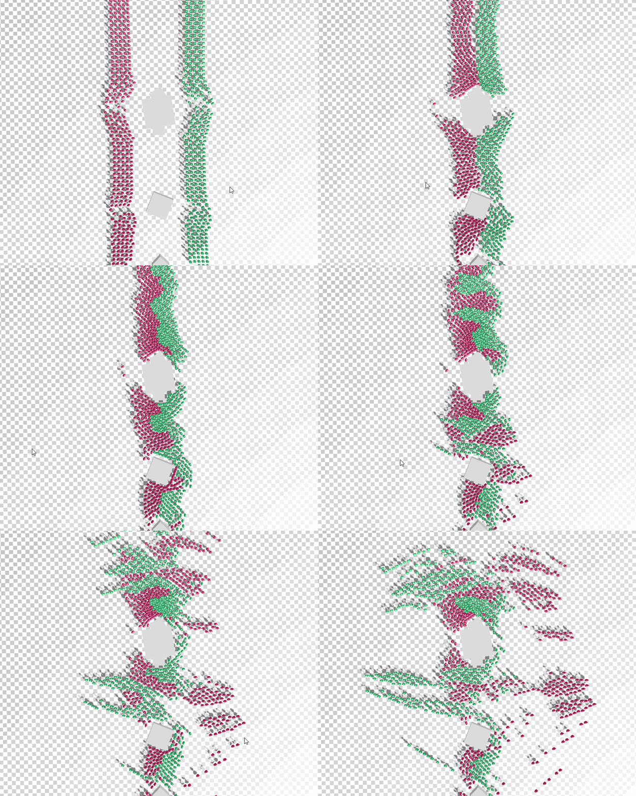
To add complexity to the scene, we support box-shaped obstacles in our implementation. The paper showcases walls as obstacles which can be modeled as line segments with short range collision constraint. We use a similar approach that considers each edge of the box as a wall constraint.
Furthermore, to enable agents to look ahead in the future and avoid obstacles, we implement an obstacle avoidance model based on OpenSteer. This affects the velocity directly in the final stage (similar to cohesion) instead of correcting the position using constraint projection. While this approach is not specifically outlined in the paper, we suspect the author having something similar based on the result produced.
| Obstacles | Bottleneck |
|---|---|
 |
 |
The author has kindly provided the parameter values used in the paper. Using them as a starting point has given us a reasonable result with very minor tweaks. The full list of parameter values used in our implementation can be found in header.compute.wgsl.
We support several different models in order to produce a visually compelling scene, which you can select via the "models" dropdown in the gui. We used the GLTFLoader from threejs to parse our gltf files, and we use the resulting gltf object to create the array buffer that we use in the WebGPU rendering pipeline. Each of the models affects the FPS proportionally to model complexity, with the duck model taking the least time, and the xbot taking the most. We were able to borrow the gltf models from the following sources:
- 'Duck' from threejs
- 'Cesium Man' from Cesium
- 'XBot' from Mixamo
- 'Ship', 'Tower', 'Garbage Truck', 'Sedan' from Kenney Assets
 |
 |
|---|---|
 |
 |
We apply basic shadow mapping to the scene based on the provided WebGPU Example. We introduce a crowd shadow render pipeline that renders the agents' depth, with respect to the light, into a depth buffer. The texture is then sampled when rendering the ground as well as the agents.
Since our test scenes vary from small/proximal to large/far, and agents' trajectories can span a large area, it is difficult to have consistently clean shadow map across the whole scene. The algorithm should be further optimized using techniques like Cascaded Shadow Mapping.
| Scene | With Shadows (fps) | Without Shadows (fps) |
|---|---|---|
| Proximal | 60 | 202 |
| Bottleneck | 42 | 58 |
| Obstacles | 23 | 33 |
| Circle | 177 | 190 |
| Circle | Dispersed |
|---|---|
 |
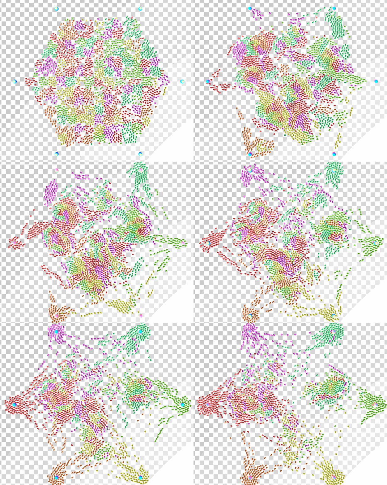 |
| Sparse | Obstacles |
|---|---|
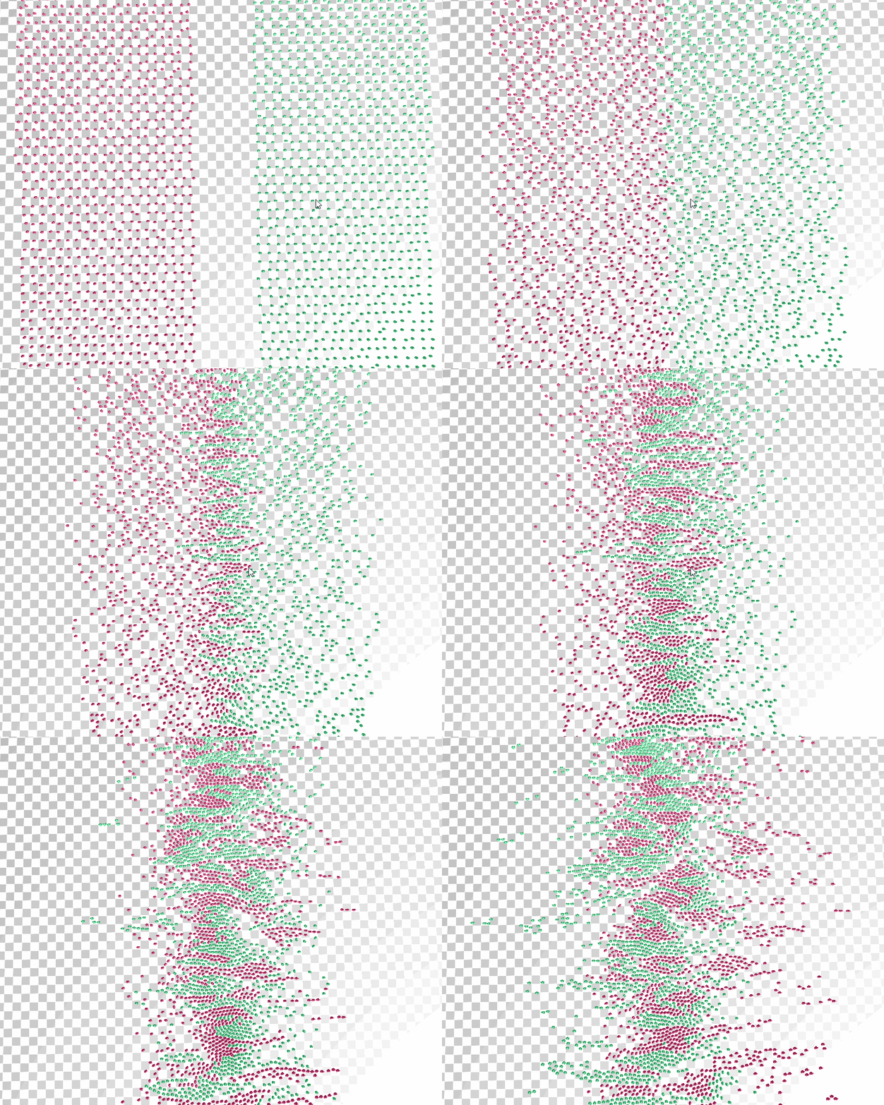 |
 |
- Animation & Skinning
- Cascaded Shadow Mapping
- Separate Grids for Short Range vs. Long Range
- WebGPU Performance Optimization
- Crowd Behavior Improvements
- Main paper of the project: PBD Crowd Simulation by Tomer Weiss et al.
- Base code from this Particles WebGPU sample by Austin Eng
- 3d-view-controls for camera manipulation
- Camera class referenced from UPenn's CIS566 base code, written by Adam Mally
- dat-gui for gui controls
- WebGPU shadow mapping example by Austin Eng
- WebGPU documentation
- Bitonic Sort wikipedia on bitonic sort
