Chronological uncertainty poses a ubiquitous challenge for sciences of the past. Nearly all of the observations we can make about past people, animals, plants, objects, and events need to be dated, and those dates are usually uncertain because the chronometric methods available come with uncertainty. Some methods come with relatively small uncertainties, like dendrochronology, which can yield age estimates with single-year errors. Others come with much higher levels of uncertainty, like radiocarbon dating, which can yield age estimates with errors ranging from decades to centuries or more. These uncertainties have long been acknowledged by the scientific community but are usually left out of formal analyses. As a result, many studies of the past contain a hidden bias. Recently, some effort has been directed toward understanding the impact that chronological uncertainty has on quantitative methods commonly used in fields like archaeology and palaeoclimatology and, consequently, the impact it has on our current understanding of the past. At the same time, statistical approaches with better handling of chronological uncertainty are being investigated and developed. One methodological avenue actively being explored involves uncertainty (error) propagation, and the R package chronup is being developed to provide access to the statistical tools produced as part of that ongoing research.
There are a few published papers so far that are directly relevant to this package. They are as follows:
-
Stewart, M., Carleton, W., Groucutt, H. (2021) DOI: 10.1038/s41467-021-21201-8
-
Carleton W. and Groucutt, H. (2020) DOI: 10.1177/0959683620981700
-
Carleton, W. (2020) DOI: 10.1002/jqs.3256
This package is currently in development and at a pre-release stage. Still, it can be installed and used in R as follows:
library(devtools)
install_github("wccarleton/chronup")
If you find bugs, have code suggestions, or feature requests, please contact me at ccarleton@protonmail.com. Once the package is ready for initial release, I will use GitHub's formal issue tracking system to handle bugs and feature requests.
Anyone interested in contributing can also feel free to contact me. Help would certainly be appreciated!
Comparing counts of radiocarbon dated samples to palaeoclimate proxies has become increasingly common in archaeology. This type of research is predicated on a popular argument about the relationship between concentrations of radiocarbon samples and human population size and/or 'activity', abstractly defined. Human activity, the argument goes, leads to increases in organic carbon contained in archaeological sediments. This is because, essentially, more people means more human remains, more fires producing charred organic carbon, more garbage pits (middens) containing organic material, more settlements with evidence of all three, etc. And so, it follows that variation through time in radiocarbon sample frequency can be expected to correlate with human population levels, broadly speaking and under certain sampling conditions---though, important caveats and inferential challenges are widely recognized. With this logic in mind, we will go over a typical chronup workflow for conducting a regression analysis involving radiocarbon dated event counts.
In lieu of analyzing real data, however, we will simulate. A simulation has two main benefits. Firstly, we can control the values of target parameters (the regression coefficients) so that we can check our answers. Secondly, using simulated dates is of course easier than obtaining real dates and for the purposes of this demonstration there is no meaningful advantage to having real ones. Real archaeological radiocarbon sample data is usually stored under controlled access and re-sharing data with identifying meta-data attached, like sample provenience, puts archaeological resources at risk. Without the provenience, however, there is no practical difference between a simulated date (randomly generated number representing a mean radiocarbon age) and a real one for our purposes here.
To simulate some radiocarbon age determinations, we can use a function called chronup::simulate_event_counts. The primary logic of the function can be divided into four steps. First, the user provides a vector of discrete solutions to a sample-generating process (e.g., population growth model) as an input along with other function parameters. Then, the function generates a random sample of true event dates from the user-generated process. Next, it produces plausible calibrated radiocarbon date densities from this sample of true event ages. And, lastly, it generates random samples of event dates from the calibrated date densities and aggregates those sampled event dates into a set of plausible event-count sequences. The primary output of the function is a matrix containing an ensemble of probable sequences where the rows of the matrix represent time and each column contains one randomly sampled probable event count series.
The chronup::simulate_event_counts function takes a number of arguments. The first three are 'process', 'times', and 'nevents'. The first argument, 'process' is expected to be a vector representing the underlying through-time variation in sample counts. It could be, for instance, solutions to a simple linear equation like y = mx + b, where 'm' is the slope of straight line and 'b' is the y-intercept for the line. Or, more likely, it will be a vector of solutions to some population model, as mentioned. The second argument, 'times' is a vector containing the corresponding time-stamps for the elements of 'process', and it is fairly self-explanatory. Typically, these times will refer to calendar years and they represent the domain of the 'process' function. Next, the 'nevents' argument is meant to contain an integer number of events in the event sample---e.g., 'nevents' might be 100, meaning 100 archaeological settlements are in the simulated dataset. Each event will have its own (not necessarily unique) time, representing the true calendar age of the corresponding event. The times are assumed to be in years before present when another argument, 'BP', is set to its default TRUE value.
The next two key arguments are 'nsamples' and 'binning_resolution'. The argument 'nsamples' defines the number of plausible event-count sequences to draw. These sequences are created by first randomly sampling density functions representing the chronological uncertainty of each randomly sampled event. Then, the random sample of event dates is aggregated into a count series. The series resolution (temporal bin width) is determined by the other key parameter, 'binning_resolution'. If the optional argument 'BP' is set to TRUE, then 'binning_resolution' must be negative because the BP scale counts up backwards in time.
Internally, chronup::simulate_event_counts calls functions from the IntCal package to produce radiocarbon dates. The chronup::simulate_event_counts first calls IntCal::calBP.14C for simulating plausible uncalibrated radiocarbon determinations from the given true calendar ages to introduce chronological uncertainty. Then, IntCal::caldist is called to calibrate the uncalibrated densities. These calibrated densities are then sampled to produce probable event count sequences, as explained.
It should be noted, though, that radiocarbon date sampling and calibration only happens when the optional argument, 'c14', is set to TRUE. It is also possible to pass uncertainty functions for each event to the chronup::simulate_event_counts directly rather than using IntCal functions or even simulated radiocarbon dates at all. An optional argument, 'chronun_matrix', can be defined with a matrix. The rows of this matrix refer to discrete times and each column to a given event. The columns should contain densities estimated at the corresponding discrete times (rows) representing the probability that the relevant event is dated to the given time.
To use the chronup::simulate_event_counts function, first load the chronup library:
library(chronup)
#> Loading required package: truncnorm
#> Loading required package: progress
#> Loading required package: pbapply
#> Loading required package: rlang
The example process will be a simple exponential function of time. To generate the discrete samples needed for the 'process' argument, we will define the number of temporal intervals ('nintervals'), a range of calendar dates ('times'), and a slope parameter ('beta'). Then, we will store discrete solutions of the exponential process in the variable 'process' and define the number of events to sample from this process ('nevents') and the number of plausible event count sequences to simulate ('nsamples'). Lastly, we call chronup::simulate_event_counts, passing all of these variables as arguments to the function.
nintervals <- 1000
times <- 5000:4001
beta <- -0.004
process <- exp(1:nintervals * beta)
nevents <- 500
nsamples <- 50000
sim_sequences <- simulate_event_counts(process = process,
                            times = times,
                            nevents = nevents,
                            nsamples = nsamples,
                            parallel = T)
#> Simulating and calibrating c14 dates.
#> Simulating event count sequences.
There are two optional arguments included in the function call above, 'bigmatrix' and 'parallel'. In practice, a very large number of plausible event count sequences should be explored in order to account for the chronological uncertainty represented by the joint-density of radiocarbon-dates for a set of events. It is also increasingly common in the academic literature for the number of radiocarbon samples analyzed to be quite large (hundreds to tens-of-thousands of dates). So, to accommodate the large number of plausible count sequences that should be drawn---which can run into the millions---the chronup package can make use of parallelization for sampling and the R package 'bigmemory' for handling large matrices. The 'bigmatrix' option was set to 'F' because the simulated dataset is reasonable small. In practice, though, many more cores may be needed to run a real analysis involving hundreds to thousands of dates and a bigmemory matrix may be required to store and manipulate millions of sampled event count sequences.
With the sampled sequences in hand, it will be useful to visualize the data. First, we can plot the event-generating process, reversing the plot axis so that time flows left-to-right:
plot(y = process,
    x = times,
    type = "l",
    xlim = c(times[1], times[length(times)]),
    xlab = "Time",
    ylab = "Process Level")
As we would expect, the process is an exponential function that decays at the rate 'beta'.
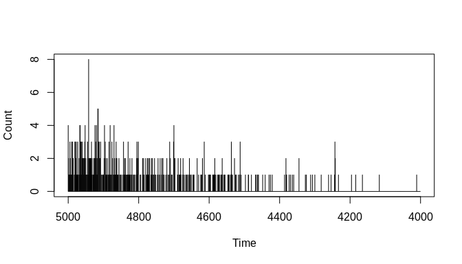
Next, we can plot the event count sample generated from this process. The chronup::simulate_event_counts function returns a list with three elements, one of which is named 'counts'. This element contains a data frame with the sampled count sequence and associated time-stamps. Plotting this count sequence shows that the simulated data appear to be a reasonable sample from the input event-generating process:
plot(y = sim_sequences$counts$Count,
    x = sim_sequences$counts$Timestamps,
    type = "h",
    xlim = c(times[1], times[length(times)]),
    xlab = "Time",
    ylab = "Count")
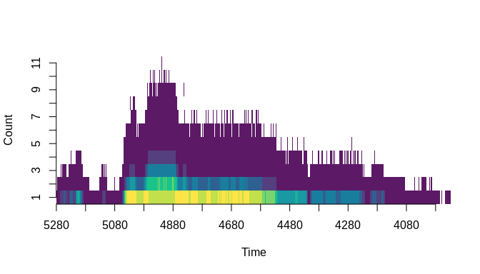
Lastly, we can plot the joint-density of event count and time in a way that includes the uncertainties involved. The chronup package provides a plotting function, chronup::plot_count_ensemble, for this purpose. It takes two main arguments, 'count_ensemble' and 'times'. The first of these is going to be the count ensemble matrix output by the simulation function we just used, and the second will be another output from that function called 'new_times'. The latter is a vector of time-stamps that correspond to the rows of the count ensemble matrix. These will be different than the original time-stamps passed to the simulation function as the argument 'times'. The differences arise because the chronological uncertainty associated with individual event times ultimately means that the span of probable time-stamps covered by the simulated event count sequence is longer than the span covered by the original event generating process---a phenomenon sometimes called 'temporal spread'.
plot_count_ensemble(count_ensemble = sim_sequences$count_ensemble,
                    times = sim_sequences$new_times)
#> NULL
In this plot, chronological uncertainty is captured by a heat map. The colours in the heatmap indicate the relative probability of count-time pairings based on the sample represented by the count ensemble. Warmer colours indicate higher relative probabilities whereas cooler colours indicate lower relative probabilities. So, it is important not to allow your eye to be fooled into following only the peaks and troughs of the plot in the y-axis dimension. The z-axis is crucial and it is represented in the plot by colour. We can see the overall shape of the event generating process represented in the plot, but it is not a perfect representation. There are features in the plot that do not reflect the true underlying process. This plot represents both event counts and chronological uncertainty about individual event times. Still, it provides useful visual information, like the fact that there is a relatively high probability (hot colours) that the count is exactly one around 5000--4800 BP, which is what we would expect given that the highest part of the exponential function used to produce the data is at 5000 BP. At the same time, though, the probability that the count is >5 in that interval is relatively low. This is also something that we would expect because the sample size is small---i.e., we only drew 100 events from the process at an annual resolution over a thousand year period, so the probability that a large number of those samples co-occurred in time often enough to create high y-axis peaks in this plot is likewise small.
With the simulated data in hand, and the plots showing what we expected to see, we can now run a simple chronup regression. The package provides a function for that purpose called chronup::regress. The regression function is Bayesian and uses an MCMC approach to uncertainty propagation. An MCMC approach to uncertainty effectively just means sampling probable values for the data, and then fitting a regression model to the samples to produce posterior distributions for the model parameters that reflect the variability in the samples. In this case, we are focusing on variability derived from chronological uncertainty about event times, but in general the sampling process could be used to incorporate any kind of uncertainty as long as we have representative distributions to draw samples from. It is also worth highlighting here that for this demonstration we are only looking at uncertainty in the event counts, the dependent variable.
The MCMC employed by chronup::regress is a basic Metropolis-Hasting algorithm. So, behind the scenes it uses random samples of potential values for the key regression model parameters and Bayes rule to estimate posterior densities for those parameter values. The algorithm chooses, for example, a random value for a regression coefficient and then calculates the likelihood of that value given the available data. It then keeps or discards that value with a given probability and tries again. Any values the algorithm keeps are stored in vectors called MCMC chains. It is these chains that will ideally contain good samples of parameter posterior distributions once the algorithm has settled on the most likely values for each parameter given the data. The regress function also includes an adaptive process for finding the best distributions from which to randomly draw potential parameter values.
The chronup::regress function takes six main arguments. The first two are 'Y' and 'X', which refer to the dependent and independent variables, respectively. Importantly, though, these will be matrices. The 'Y' argument in our example will be the event count ensemble we produced with the simulation above and the 'X' value will be a matrix where each column is just time indexes from 1 to 1000 representing the passage of time. Each column in 'Y', remember, is a probable event count sequence, and potentially each column in 'X' could be a probable series for the independent variable. The MCMC in the regress function will then walk over these two matrices as the simulation proceeds. Each time the algorithm draws new potential values for the regression model parameters, it will also be selecting a new probable event count sequence and a new probable series for the independent variable(s).
The third argument in the regress function is 'model'. This argument takes a string and can, as of the time of writing, be either 'pois' or 'nb'. These options refer to the two types of count models currently available in the regress function. The first refers to a Poisson ('pois') regression model and the second to a Negative Binomial ('nb') regression model. As has been explained elsewhere, the Negative Binomial distribution comes with advantages for modelling radiocarbon-dated event counts. In particular, it can be adjusted to account better for temporal spread than a simpler Poisson model. This type of model has been referred to as a Negative Binomial Radiocarbon-dated Event Count (NB-REC) model. Here, however, we will focus on the Poisson model because its simplicity makes for faster computation.
The last three arguments for the regress function are 'startvals', 'startscales', and 'adapt'. The 'startvals' argument takes a vector of starting values for the regression model parameters. In the case of the 'nb' model, this vector must contain one element for each regression coefficient (including an intercept if one is needed) and then one element for each 'p' parameter of a standard Negative Binomial distribution for each observation in the count sequence. So, there would be as many 'p' parameters as there are rows in 'Y'. This is not the case with the Poisson model, which has only the usual regression coefficients to worry about. The 'startscales' argument also takes a vector of values. Each element is used as the scale (variance) for the proposal distributions associated with the model's parameters---these are the distributions that the MCMC samples at random when trying different values for each parameter. One scale value has to be given for each parameter in the model, which means that 'startscales' will have the same length as 'startvals'. Finally, the 'adapt' argument is a logical (TRUE/FALSE) value that indicates whether the 'startscales' provided should be adapted by the algorithm. When it is TRUE, the algorithm will shrink/grow the scales for each parameter's proposal distribution depending on the average rate at which it has been accepting potential parameter values.
The number of iterations run during the MCMC can be set with an optional 'niter' parameter. But, if left to its default 'NULL' value, the number of iterations will correspond to the number of columns in the 'Y' matrix. So, for a longer simulation that accounts for more chronological uncertainty, we would randomly sample more probable dependent and independent variable sequences.
As mentioned, for this short demonstration we are only considering chronological uncertainty in the dependent count variable. The 'X' argument is a matrix, though, and so can be used to propagate uncertainties in the independent variables as well. For now, we will simply create a matrix for 'X' that has only cloned columns each containing a copy of a vector representing time. At first, we will use the full interval of time covered by the sampled event count sequences that was returned by the simulation function. We will also include an intercept, even though the original process did not. The intercept will be represented by a column of 1s.
In order for the 'regress' function to work, it is necessary that 'Y' and 'X' have an equal number of columns, or that 'X' has a number of columns equal to an integer multiple of 'Y's number of columns. This is because the algorithm will be selecting a column from 'Y' and one or more columns from 'X' in every iteration of the MCMC. The logic here begin that these pairings, one probable 'Y' with one probable 'X', represents one of the probable combinations of the dependent and independent variable(s) given the uncertainties in both. So, in the simplest case of one dependent and one independent variable, the 'Y' and 'X' matrices must have an equal number of columns. But, if an intercept is included, then for every probable dependent--independent pairing there will be one 'Y' and two 'X' columns, the later including a column for the intercept and a column for a probable series of measures of the independent variable. More independent variables will necessarily mean there needs to be more columns in 'X', but the total number of 'X' columns will always be an integer multiple of the number of columns in 'Y'. That way, each pairing contains a set of realizations from the same set of independent and dependent variables. The following code creates the 'Y' and 'X' matrices:
Y <- sim_sequences$count_ensemble
n <- dim(Y)[1]
x0 <- rep(1, n)
x1 <- 1:n
X <- matrix(
        rep(c(x0,x1), nsamples),
        nrow = n)

dim(Y)
#> [1]  1354 50000
dim(X)
#> [1]   1354 100000

Y[1:5, 1:10]
#>      [,1] [,2] [,3] [,4] [,5] [,6] [,7] [,8] [,9] [,10]
#> [1,]    0    0    0    0    0    0    0    0    0     0
#> [2,]    0    0    0    0    0    0    0    0    0     0
#> [3,]    0    0    0    0    0    0    0    0    0     0
#> [4,]    0    0    0    0    0    0    0    0    0     0
#> [5,]    0    0    0    0    0    0    0    0    0     0
X[1:5, 1:10]
#>      [,1] [,2] [,3] [,4] [,5] [,6] [,7] [,8] [,9] [,10]
#> [1,]    1    1    1    1    1    1    1    1    1     1
#> [2,]    1    2    1    2    1    2    1    2    1     2
#> [3,]    1    3    1    3    1    3    1    3    1     3
#> [4,]    1    4    1    4    1    4    1    4    1     4
#> [5,]    1    5    1    5    1    5    1    5    1     5
Then, the 'startvals' and 'startscales' parameters should be set. If no 'startvals' are provided, though, the function will select some naive ones. In this case we will be agnostic about both (bear in mind that startscales must be positive and non zero):
startvals <- c(0,0)
startscales <- c(0.1, 0.0002)
Next, call the 'chronup::regress' function with the previously defined variables passed as the appropriate arguments. As the code below indicates, we will fun the MCMC with the 'adapt' argument 'TRUE' so that we can find better 'startvals' and 'startscales':
mcmc_samples_adapt <- regress(Y = Y,
                            X = X,
                            model = "pois",
                            startvals = startvals,
                            scales = startscales,
                            adapt = T)
With 'adapt' set to TRUE, the 'regress' function returns a list with three elements. One is a matrix containing the MCMC chains---each model parameter is represented by a separate column. The second is a matrix containing acceptance rates for all parameters recorded throughout the simulation at regular intervals (defined by other 'regress' function arguments detailed in the manpage for the function). The last element is a matrix containing the scales tried and used by the algorithm. With this information we can run 'regress' again, but use adapted estimates for the new startvals and startscales, which should improve the convergence of the MCMC leading to better samples of posterior distributions with fewer iterations overall. The MCMC chain samples produced with 'adapt' set to 'TRUE', however, should be discarded as burn-in before further analyses.
So, now we can establish new startvals and startscales given the results of the adaptive MCMC. We will discard some number of samples as burn-in (say, the first 20%) and then use the average of the remaining samples for the new values:
burnin <- floor(dim(mcmc_samples_adapt$samples)[1] * 0.1)
indeces <- seq(burnin, dim(mcmc_samples_adapt$samples)[1], 1)
new_startvals <- colMeans(mcmc_samples_adapt$samples[indeces,])

burnin <- floor(dim(mcmc_samples_adapt$scales)[1] * 0.1)
indeces <- seq(burnin, dim(mcmc_samples_adapt$scales)[1], 1)
new_startscales <- colMeans(mcmc_samples_adapt$scales[indeces,])

mcmc_samples <- regress(Y = Y,
                        X = X,
                        model = "pois",
                        startvals = new_startvals,
                        scales = new_startscales,
                        adapt = F)

head(mcmc_samples)
#>            [,1]         [,2]
#> [1,] -0.2754904 -0.001234745
#> [2,] -0.2754904 -0.001234745
#> [3,] -0.2754904 -0.001234745
#> [4,] -0.2803615 -0.001234745
#> [5,] -0.2803615 -0.001234745
#> [6,] -0.2803615 -0.001234745
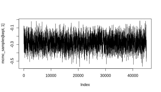
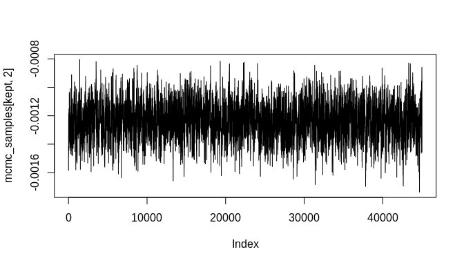
When 'adapt' is set to 'FALSE', the function returns the MCMC chains. With enough iterations, the chains will likely contain good samples of the posterior distributions corresponding to the model's parameters. These can be inspected further with standard tools, including those in the 'coda' MCMC package. Here will will simply plot the chains as line-plots and then plot some density estimates to get a quick look at the results:
burnin <- floor(dim(mcmc_samples)[1] * 0.1)
kept <- seq(burnin, dim(mcmc_samples)[1], 1)

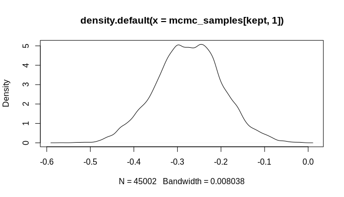
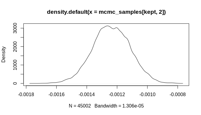
plot(mcmc_samples[kept, 1], type = "l")plot(mcmc_samples[kept, 2], type = "l")plot(density(mcmc_samples[kept, 1]))plot(density(mcmc_samples[kept, 2]))As the plots show, the chains are not fully stable and the density estimates are biased, but these indicators of poor convergence are the result of too few MCMC iterations. With more iterations, the chains will stabilize and well-behaved density estimates can be obtained.
Still, it is important to highlight that the posterior estimate for the key rate parameter---'beta'---is biased toward zero. This attenuation is a known effect of chronological uncertainty on count models. The regression does, however, produce an estimate with the correct sign (negative in this example) and the posterior distribution is sufficiently far from zero that the result could be considered statistically significant at the 99% confidence level or higher. Stable MCMC chains would be required in order to get a suitable confidence estimate, of course.
The bias can be reduced further if we limit the analysis to the temporal span of the original simulation process. In practice, a similar subsetting of the data could be justified by gathering data outside a given temporal interval of analytical interest and/or limiting analyses to a subinterval of the available data. It may be a debatable decision in any given case and more research is required. Nevertheless, for the sake of this demonstration, the code below subsets the simulated data, limiting the analysis to the original temporal interval (5000--4001 BP):
subinterval <- which(sim_sequences$new_times <= 5000 &
                    sim_sequences$new_times >= 4001)

mcmc_samples_adapt <- regress(Y = Y[subinterval,],
                            X = X[subinterval,],
                            model = "pois",
                            startvals = startvals,
                            scales = startscales,
                            adapt = T)

burnin <- floor(dim(mcmc_samples_adapt$samples)[1] * 0.1)
indeces <- seq(burnin, dim(mcmc_samples_adapt$samples)[1], 1)
new_startvals <- colMeans(mcmc_samples_adapt$samples[indeces,])

burnin <- floor(dim(mcmc_samples_adapt$scales)[1] * 0.1)
indeces <- seq(burnin, dim(mcmc_samples_adapt$scales)[1], 1)
new_startscales <- colMeans(mcmc_samples_adapt$scales[indeces,])

mcmc_samples <- regress(Y = Y[subinterval,],
                        X = X[subinterval,],
                        model = "pois",
                        startvals = new_startvals,
                        scales = new_startscales,
                        adapt = F)

head(mcmc_samples)
#>          [,1]         [,2]
#> [1,] 1.590566 -0.003719868
#> [2,] 1.590566 -0.003719868
#> [3,] 1.590566 -0.003719868
#> [4,] 1.590566 -0.003719868
#> [5,] 1.625469 -0.003719868
#> [6,] 1.625469 -0.003719868
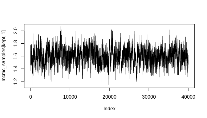
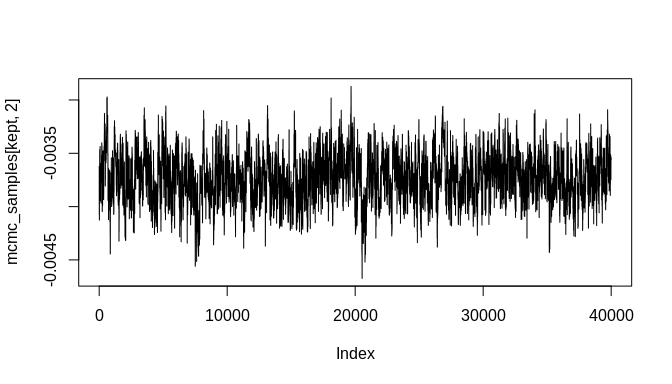
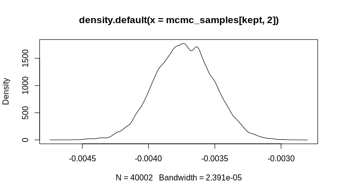
As the plots below indicate, the initial bias is significantly reduced and the true parameter estimate ('beta', which was set to -0.004 above) is within the 95% credible interval of the estimated posterior distribution. Again, many more MCMC iterations will be required in order to arrive at good estimates of posterior distributions for the model parameters. The additional iterations will come from increasing the number of randomly sampled probable event count sequences. As a result, an even better estimate of the overall chronological uncertainty in the data can be obtained and then propagated up to the regression model parameter estimates. Additionally, using a Negative-Binomial (NB-REC) model instead would further reduce the bias, especially if the complete time domain of the event count ensemble is being analyzed instead of a subinterval.
burnin <- floor(dim(mcmc_samples)[1] * 0.2)
kept <- seq(burnin, dim(mcmc_samples)[1], 1)

plot(mcmc_samples[kept, 1], type = "l")plot(mcmc_samples[kept, 2], type = "l")plot(density(mcmc_samples[kept, 1]))plot(density(mcmc_samples[kept, 2]))
