usfertilizer

County-lelel nutrients data from 1945 to 2012 in USA

Usfertilizer summarized the estimated county level data from USGS of USA and provided a clean version using Tidyverse.

Please note that USGS does not endorse this package. Also data from 1986 is not available for now.

Introduction of data sources and availability

The data used in this package were original compiled and processed by United States Geographic Services (USGS). The fertilizer data include the application in both farms and non-farms for 1945 through 2012. The folks in USGS utilized the sales data of commercial fertilizer each state or county from the Association of American Plant Food Control Officials (AAPFCO) commercial fertilizer sales data. State estimates were then allocated to the county-level using fertilizer expenditure from the Census of Agriculture as county weights for farm fertilizer, and effective population density as county weights for nonfarm fertilizer. The data sources and other further information are availalbe in Table below.

Dataset name	Temporal coverage	Source	Website	Comments
Fertilizer data before 1985	1945 - 1985	USGS	Link	Only has farm data.
Fertilizer data after 1986	1986 - 2012	USGS	Link	Published in 2017.
County background data	2010	US Census	Link	Assume descriptors of counties do not change.
Manure data before 1997	1982 - 1997	USGS	Link	Manual data into farm every five years
Manure data in 2002	2002	USGS	Link	Published in 2013
Manure data in 2007 and 2012	2007 & 2012	USGS	Link	Published in 2017

Installation

Install the stable version via CRAN, just run:

install.packages("usfertilizer")

You can also install the package via my Github Repository.

# install.package("devtools")   #In case you have not installed it.
devtools::install_github("wenlong-liu/usfertilizer")

Get started

Import data and related libraries

require(usfertilizer)
require(tidyverse)
data("us_fertilizer_county")

Summary of the dataset

The dataset, named by us_fertilizer_county, contains 625580 observations and 11 variables. Details are available by using ?us_fertilizer_county.

glimpse(us_fertilizer_county)
#> Observations: 625,580
#> Variables: 12
#> $ FIPS       <chr> "01001", "01003", "01005", "01007", "01009", "01011...
#> $ State      <chr> "AL", "AL", "AL", "AL", "AL", "AL", "AL", "AL", "AL...
#> $ County     <chr> "Autauga", "Baldwin", "Barbour", "Bibb", "Blount", ...
#> $ ALAND      <dbl> 1539582278, 4117521611, 2291818968, 1612480789, 166...
#> $ AWATER     <dbl> 25775735, 1133190229, 50864716, 9289057, 15157440, ...
#> $ INTPTLAT   <dbl> 32.53638, 30.65922, 31.87067, 33.01589, 33.97745, 3...
#> $ INTPTLONG  <dbl> -86.64449, -87.74607, -85.40546, -87.12715, -86.567...
#> $ Quantity   <dbl> 1580225, 6524369, 2412372, 304592, 1825118, 767573,...
#> $ Year       <chr> "1987", "1987", "1987", "1987", "1987", "1987", "19...
#> $ Nutrient   <chr> "N", "N", "N", "N", "N", "N", "N", "N", "N", "N", "...
#> $ Farm.Type  <chr> "farm", "farm", "farm", "farm", "farm", "farm", "fa...
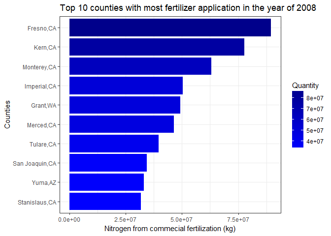
#> $ Input.Type <chr> "Fertilizer", "Fertilizer", "Fertilizer", "Fertiliz...

Examples

Example 1: Find out the top 10 counties with most nitrogen appliation in 2008.

# plot the top 10 nitrogen application in year 2008.
# Reorder to make the plot more cleanner.
year_plot = 2008
us_fertilizer_county %>%
  filter(Nutrient == "N" & Year == year_plot & Input.Type == "Fertilizer" ) %>%
  top_n(10, Quantity) %>%
  ggplot(aes(x=reorder(paste(County,State, sep = ","), Quantity), Quantity, fill = Quantity))+
  scale_fill_gradient(low = "blue", high = "darkblue")+
  geom_col()+
  ggtitle(paste("Top 10 counties with most fertilizer application in the year of", year_plot)) + 
  scale_y_continuous(name = "Nitrogen from commecial fertilization (kg)")+
  scale_x_discrete(name = "Counties")+
  coord_flip()+
  theme_bw()

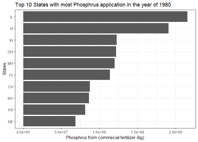
Example 2: Find out the top 10 states with most nitrogen appliation in 1980.

# plot the top 10 states with P application in year 1980.
# Reorder to make the plot more cleanner.
year_plot = 1980
us_fertilizer_county %>%
  filter(Nutrient == "P" & Year == 1980 & Input.Type == "Fertilizer") %>% 
  group_by(State) %>% 
  summarise(p_application = sum(Quantity)) %>% 
  as.data.frame() %>% 
  top_n(10, p_application) %>%
  ggplot(aes(x=reorder(State, p_application), p_application))+
  scale_fill_gradient(low = "blue", high = "darkblue")+
  geom_col()+
  ggtitle(paste("Top 10 States with most Phosphrus application in the year of", year_plot)) + 
  scale_y_continuous(name = "Phosphrus from commecial fertilizer (kg)")+
  scale_x_discrete(name = "States")+
  theme_bw()+
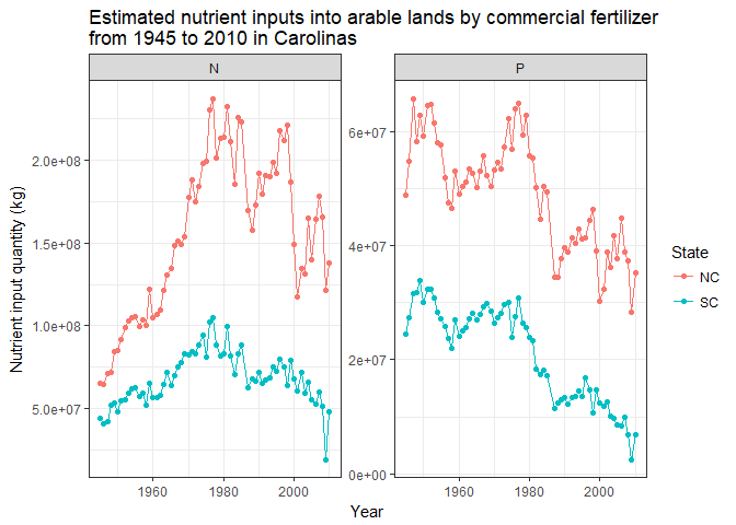
  coord_flip()

Example 3: Plot the N and P input into farms for NC and SC from 1945 to 2010

year_plot = seq(1945, 2010, 1)
states = c("NC","SC")

us_fertilizer_county %>% 
  filter(State %in% states & Year %in% year_plot &
           Farm.Type == "farm" & Input.Type == "Fertilizer") %>% 
  group_by(State, Year, Nutrient) %>% 
  summarise(Quantity = sum(Quantity, na.rm = T)) %>% 
  ggplot(aes(x = as.numeric(Year), y = Quantity, color=State)) +
  geom_point() +
  geom_line()+
  scale_x_continuous(name = "Year")+
  scale_y_continuous(name = "Nutrient input quantity (kg)")+
  facet_wrap(~Nutrient, scales = "free", ncol = 2)+
  ggtitle("Estimated nutrient inputs into arable lands by commercial fertilizer\nfrom 1945 to 2010 in Carolinas")+
  theme_bw()

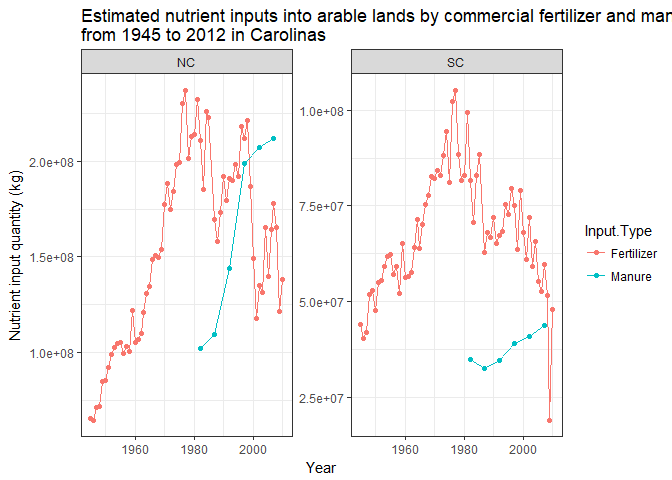
Example 4: Plot the N input into farms from fertilizer and manure for NC and SC from 1945 to 2012

us_fertilizer_county %>% 
  filter(State %in% states & Year %in% year_plot &
           Farm.Type == "farm" & Nutrient == "N") %>% 
  group_by(State, Year, Input.Type) %>% 
  summarise(Quantity = sum(Quantity, na.rm = T)) %>% 
  ggplot(aes(x = as.numeric(Year), y = Quantity, color=Input.Type)) +
  geom_point() +
  geom_line()+
  scale_x_continuous(name = "Year")+
  scale_y_continuous(name = "Nutrient input quantity (kg)")+
  facet_wrap(~State, scales = "free", ncol = 2)+
  ggtitle("Estimated nutrient inputs into arable lands by commercial fertilizer and manure\nfrom 1945 to 2012 in Carolinas")+
  theme_bw()

Comments and Questions.

If you have any problems or questions, feel free to open an issue here.

Lisence

GPL

Code of conduct

Please note that this project is released with a Contributor Code of Conduct. By participating in this project you agree to abide by its terms.

Preferred citation

Wenlong Liu (2018). usfertilizer: County-Level Estimates of Fertilizer Application in USA. R package version 0.1.5. https://CRAN.R-project.org/package=usfertilizer. DOI:10.5281/zenodo.1292843