Joyce Robbins 2021-10-28
library(tidyverse)
library(wonderapi)This package makes it easier to use the CDC Wonder API. It does so by employing hidden default query lists and lookup tables, allowing users to focus only on the variables they’re interested in obtaining, and to write queries using human readable names rather than numeric codes.
getData()
- converts the user’s parameter requests to codes
- adds these codes to the default query list
- calls
wondr::make_queryto obtain query results - processes the results
- returns a tidy data frame
Note that queries for mortality and births statistics from the National Vital Statistics System cannot limit or group results by any location field, such as Region, Division, State or County, or Urbanization (urbanization categories map to specific geographic counties). See: https://wonder.cdc.gov/wonder/help/WONDER-API.html for more information.
mylist <- list(list("And By", "Gender"))
mydata0 <- getData(TRUE, "Detailed Mortality", mylist)
mydata0 %>% head()## # A tibble: 6 × 5
## Year Gender Deaths Population `Crude Rate`
## <dbl> <chr> <dbl> <dbl> <dbl>
## 1 1999 Female 1215860 142237295 855.
## 2 1999 Male 1175183 136802873 859
## 3 2000 Female 1225706 143368343 855.
## 4 2000 Male 1177289 138053563 853.
## 5 2001 Female 1232913 145077463 850.
## 6 2001 Male 1183090 139891492 846.
show_databases() displays available databases by name and code:
wonderapi::show_databases()## # A tibble: 5 × 2
## label name
## <chr> <chr>
## 1 Natality for 1995 - 2002 D10
## 2 Natality for 2003 - 2006 D27
## 3 Natality for 2007 - 2019 D66
## 4 Detailed Mortality D76
## 5 Heat Wave Days D104
More databases will be added in the future.
The best way to become familiar with CDC Wonder API options is to use the web interface: https://wonder.cdc.gov, as the options available through the API are nearly identical. The greatest difference is that location variables are not available through the API.
This package is not on CRAN. It can be installed from Github with the
devtools package:
devtools::install_github("socdataR/wonderapi", build_vignettes = TRUE)(The vignettes are an important component of the package as the
codebooks are stored as vignettes, so be sure to include
build_vignettes = TRUE.)
Queries are composed of parameter name-value pairs. Setting up a query
without assistance is complex because the query must be submitted as an
.xml file with a long list of required parameters, such as here
(Example
1)
and here (Example
2).
The point of the package is to prevent your having to create requests in
this form. It relies on the wondr package which creates converts R
lists to xml and makes the query. The value of this package is in the
“pre” and “post” stages of the query, that is, the processes of setting
up the query and tidying the results.
Codebooks are provided as package vignettes to allow the user to conveniently look up the names and values of available parameters in each dataset. They may be accessed quickly by typing:
> ??codebookin the console, or searching for “codebook” in the Help window. The
codebooks are an important contribution of the package and are not
provided by the CDC. They are generated automatically by this
script,
which scrapes the CDC Wonder web interface form, and displays parameter
names and values in human readable form. The benefit of this method is
the ability to quickly produce and update codebook vignettes that
closely follow the web interface, with parameters appearing in the same
order. It also means, however, that the codebooks contain more
information than the typical user needs to submit a query. Most users
will only need Group By variables (codes beginning with “B_”), Measures
(codes beginning with “M_”), and Limiting Variables (codes beginning
with “V_”).
Although some of the parameter names are long and/or awkward, for the sake of consistency, we follow the CDC names exactly. The only exception is that any content that appears in parentheses should be dropped. For example, “Fertility Rate” can be substituted for “M_5”, but “Fertility Rate (Census Region, Census Division, HHS Region, State, County, Year, Age of Mother, Race) cannot.
To facilitate the process of designing a query list, this package relies
on default query lists. Each default query is set to request a single
Group By Results parameter, generally set to "Year". It is set to
request the Measures that are listed as default Measures on the web
interface (i.e. Births for the Births
dataset; Deaths,
Population and Crude Rate for the Detailed Mortality
dataset.) To see the
default settings, perform a query request without specifying a
querylist:
natdata <- getData(TRUE, "Natality for 2007 - 2019")
natdata %>% head()
## # A tibble: 6 × 2
## Year Births
## <dbl> <dbl>
## 1 2007 4316233
## 2 2008 4247694
## 3 2009 4130665
## 4 2010 3999386
## 5 2011 3953590
## 6 2012 3952841
dmdata <- getData(TRUE, "Detailed Mortality")
dmdata %>% head()
## # A tibble: 6 × 4
## Year Deaths Population `Crude Rate`
## <dbl> <dbl> <dbl> <dbl>
## 1 1999 2391043 279040168 857.
## 2 2000 2402995 281421906 854.
## 3 2001 2416003 284968955 848.
## 4 2002 2443030 287625193 849.
## 5 2003 2447946 290107933 844.
## 6 2004 2397269 292805298 819.
The default lists were prepared based on CDC examples, but we make no claim that they are error free. If you have any suggestions for improving them, please make a pull request on Github or send an email to Joyce Robbins. The default lists are available here.
There are different types of parameters. Most critical are Group Results By and Measures. The Group Results By parameters serve as keys for grouping the data; the maximum number of Group Results By parameters is five. Limiting Variables may also be used to constrain results behind the scenes.
To make changes to the default list, first create a list of lists, wherein each nested list is a name-value pair. For example, the following changes the first (and currently only) “Group Results By” variable to Weekday:
mylist <- list(list("Group Results By", "Weekday"))
mydata <- getData(TRUE, "Detailed Mortality", mylist)
mydata %>% head()## # A tibble: 6 × 4
## Weekday Deaths Population `Crude Rate`
## <chr> <dbl> <chr> <chr>
## 1 Sunday 7575854 Not Applicable Not Applicable
## 2 Monday 7638335 Not Applicable Not Applicable
## 3 Tuesday 7586763 Not Applicable Not Applicable
## 4 Wednesday 7585543 Not Applicable Not Applicable
## 5 Thursday 7596742 Not Applicable Not Applicable
## 6 Friday 7711294 Not Applicable Not Applicable
As the set up is slightly different depending on the parameter type, more details on setting up the name-value pairs by parameter types are provided below.
Each dataset allows for fixed number (5 or fewer) Group By variables,
codes for which are "B_1", "B_2", "B_3", etc. "Group By Results" may
be substituted for "B_1" and "And By" for "B_2". "And By” may
not, however, be substituted for "B_3" on to avoid ambiguity (this
may change in the future.) Values – in this case, the Group By variables
– may be specified by code or human readable name. The following, thus,
are equivalent:
## not run
mylist <- list(list("B_1", "D66.V2"))
mylist <- list(list("Group Results By", "Race"))
mylist <- list(list("B_1", "Race"))
mylist <- list(list("Group Results By", "D66.V2"))
See the appropriate codebook for all Group By options.
Measures do not need values; it is sufficient to specify a name only:
mylist <- list(list("Group Results By", "Marital Status"),
               list("And By", "Year"),
               list("Average Age of Mother", ""))
mydata2 <- getData(TRUE, "Natality for 2007 - 2019", mylist)
mydata2 %>% head()## # A tibble: 6 × 4
## `Marital Status` Year Births `Average Age of Mother`
## <chr> <dbl> <dbl> <dbl>
## 1 Married 2007 2601186 29.5
## 2 Married 2008 2521128 29.6
## 3 Married 2009 2437007 29.7
## 4 Married 2010 2365915 29.8
## 5 Married 2011 2345817 29.9
## 6 Married 2012 2343222 30.0
Queries can be constrained with parameters that limit results in the background. For example, if you’re only interested in February births, you may choose to limit results to February as follows, rather than grouping by Month:
mylist <- list(list("Month", "2"))
getData(TRUE, "D66", mylist)
## # A tibble: 13 × 2
## Year Births
## <dbl> <dbl>
## 1 2007 326891
## 2 2008 338521
## 3 2009 316641
## 4 2010 301994
## 5 2011 297961
## 6 2012 304505
## 7 2013 291748
## 8 2014 298404
## 9 2015 298058
## 10 2016 306015
## 11 2017 289054
## 12 2018 284250
## 13 2019 279963
Note that values for Limiting Variables must be entered as codes; in this case “2” rather than “February.” We hope to add capability for human readable values in the future.
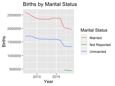
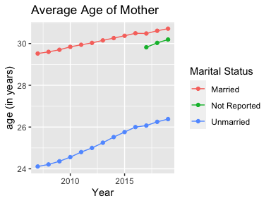
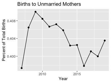
By returning a tidy data frame, the query results are ready to be plotted without any additional data manipulation:
ggplot(mydata2, aes(x = Year, y = Births, color = `Marital Status`)) +
geom_line() + ggtitle("Births by Marital Status")ggplot(mydata2, aes(x = Year, y = `Average Age of Mother`,
color = `Marital Status`)) + geom_line() +
geom_point() + ylab("age (in years)") +
ggtitle("Average Age of Mother")mydata2 <- mydata2 %>%
select(-`Average Age of Mother`) %>%
spread(key = `Marital Status`, value = `Births`) %>%
mutate(Total = Married + Unmarried)
ggplot(mydata2, aes(x = Year, y = Unmarried / Total)) + geom_line() +
geom_point() + ggtitle("Births to Unmarried Mothers") +
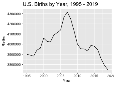
ylab("Percent of Total Births")Some of the datasets, such as the Births, are divided into multiple
databases by time period. wonderapi makes it easy to combine the data
into one data frame. (Care needs to be taken as the variables are not
identical in all. For example, the 1995 - 2002 dataset does not have any
measure options; it only returns number of births. To find out what’s
available, see the codebooks (>??codebook) and crosscheck with the
CDC Wonder API web interface.)
births <- rbind(getData(TRUE, "Natality for 1995 - 2002"),
                getData(TRUE, "Natality for 2003 - 2006"),
                getData(TRUE, "Natality for 2007 - 2019"))
ggplot(births, aes(Year, Births)) + geom_line() +
ggtitle("U.S. Births by Year, 1995 - 2019")The main source of errors is improper query requests. The wonderapi
has limited ability to catch problems before the query request is made.
It checks the list of parameter names and will reject the name-value
pair if the name, either in code or human readable form, is not
recognized. (Checking for value problems will be added in the future.)
Here is an example of an unrecognized parameter name:
mydata3 <- getData(TRUE, "Detailed Mortality",
        list(list("Suspect", "Mrs. Peacock")))
## Ignoring: "Suspect",...(not recognized)
mydata3 %>% head()## # A tibble: 6 × 4
## Year Deaths Population `Crude Rate`
## <dbl> <dbl> <dbl> <dbl>
## 1 1999 2391043 279040168 857.
## 2 2000 2402995 281421906 854.
## 3 2001 2416003 284968955 848.
## 4 2002 2443030 287625193 849.
## 5 2003 2447946 290107933 844.
## 6 2004 2397269 292805298 819.
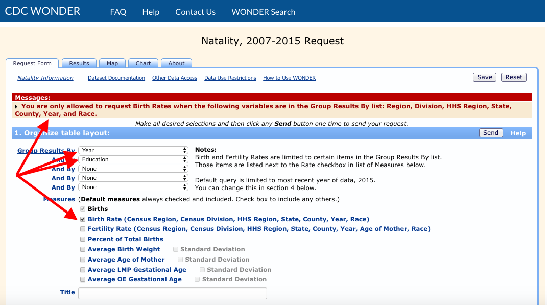
Errors due to the constraints of the CDC Wonder API are more difficult to catch since there are many quirky rules and it is currently beyond the scope of this package to check for them. The following, for example, appears to be a reasonable request, but results in an error:
mylist <- list(list("And By", "Education"),
               list("Birth Rate", ""))
mydata4 <- getData(TRUE, "Natality for 2007 - 2019", mylist)
## Error in wondr::make_query(querylist, dbcode): Internal Server Error (HTTP 500).
In this case, the best approach is to visit the CDC Wonder API web interface and try the same query. If all goes well, you will receive more detailed information on what went wrong:
We learn that we can’t include “Education” if we request the “Birth Rate” measure. If we try again with “Bridged Race” instead of “Education”, it works:
mylist <- list(list("And By", "Mother's Bridged Race"),
               list("Birth Rate", ""))
mydata5 <- getData(TRUE, "Natality for 2007 - 2019", mylist)
mydata5 %>% head()## # A tibble: 6 × 5
## Year `Mother's Bridged Race` Births `Total Population` `Birth Rate`
## <dbl> <chr> <dbl> <dbl> <dbl>
## 1 2007 American Indian or Alaska Native 49443 3829898 12.9
## 2 2007 Asian or Pacific Islander 254488 15559373 16.4
## 3 2007 Black or African American 675676 40451108 16.7
## 4 2007 White 3336626 241390828 13.8
## 5 2008 American Indian or Alaska Native 49537 3983929 12.4
## 6 2008 Asian or Pacific Islander 253185 16094699 15.7
