tapas R-package

Rationale

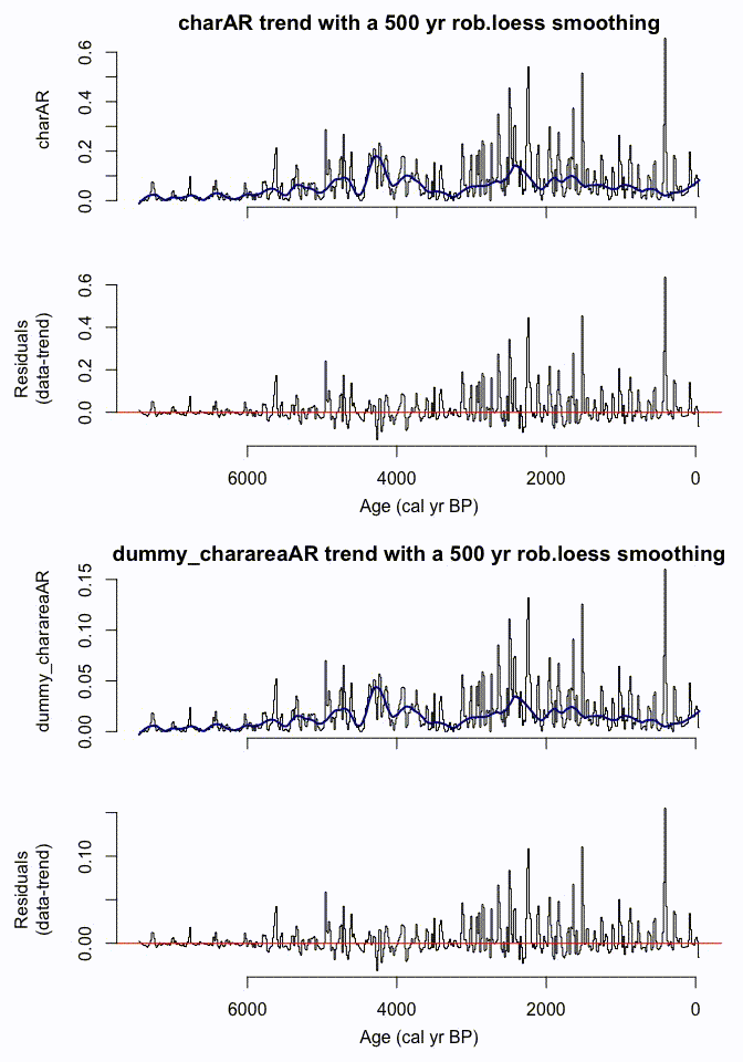
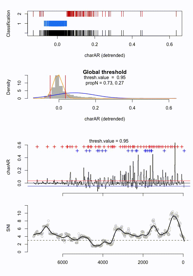
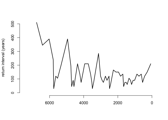
The set of functions gathered under the hood of tapas is meant to be used for analyzing paleoecological records, when the goal is to estimate the long-term Trend and detect Peaks to reconstruct the occurrence, the return intervals, and the magnitude of distinct events.

tapas builds on CharAnalysis (https://github.com/phiguera/CharAnalysis), a software for analyzing sediment-charcoal records written in and compiled with Matlab 7.0 by Phil Higuera (Higuera et al., 2009), with significant input by (amongst others) Patrick Bartlein (U of OR), Daniel Gavin (U of OR), Jennifer Marlon, and Ryan Kelly.

Two main reasons led to the development of tapas. Firstly, as R is an open source product, modifying the program to suit individual needs may be more straightforward. Secondly, an integration and inter-operability with other existing R-packages may allow using peak-detection analysis in conjunction with other workflows and types of paleoecological records (see for instance (Cagliero et al., 2021)).

Usage

A typical workflow of the peak-detection analysis includes the following steps (Higuera et al., 2011):

1.) resample the record to equally spaced sampling intervals in time (years), a procedure also called “binning”
2.) decompose the resampled record into a long-term trend (background component) and peaks (peak component)
3.) screen the peak component to distinguish signal from noise using
- 3.1 a unique global 2-component Gaussian mixture model, or
- 3.2 local 2-component Gaussian mixture models,
- 3.3 and eventually also screen the peak component using a minimum-count test,
4.) evaluate the suitability of the record for peak-detection analysis using the signal-to-noise index (Kelly et al., 2011).

tapas performs steps 1.) and 2.) for several variables of one dataset type (e.g. different estimates of charcoal abundance) in one go. Instead, steps 3.) and 4.) are performed for one user-selected variable.

To run your own data, make a new folder within an umbrella folder, and save it under a name, e.g., Data-In. Then place a file (e.g., MyData.csv) in that folder. The input data file will contain the sample depths, sample ages, sample volume, and the variable(s). The file should have the following formatting: It has headers and at least six fields. The first five columns will report the metadata for the samples, the subsequent columns contain the variable(s) to be analysed (e.g., the abundance of charcoal pieces).

CmTop	CmBot	AgeTop	AgeBot	Volume	variable1	variable2	…	nth-variable
0.5	1	-42	-24	3	8	0.01	…	…
1	1.5	-24	5	3	18	0.005	…	…

The depths and ages should be arranged in ascending order.

Load the data into the R environment

MyData <- read.csv(“./Data-In/MyData.csv”)

Installation

Install the development version of tapas with:

# library(devtools)
devtools::install_github("wfinsinger/tapas")

The check_pretreat() function can be used to verify the input data is formatted correctly. If the samples in the input file are not contiguous, the check_pretreat() function will add rows for the missing samples. Should the dataset contain samples that were deposited in a very short amount of time (e.g., slumps, tephras), for which AgeTop = AgeBot, these samples will be flagged and removed, and a new depth scale will be created to replace the original one.

MyData <- check_pretreat(Mydata)

The functions can either be run individually and step wise, or the wrapper function peak_detection() can be used to perform an analysis including steps from 1.) to 4.) in one go.

For instance, to analyse the MyData data set for variable1:

MyData_peaks <- peak_detection(series = MyData, proxy = “variable1”)

Individual output plots can be generated with dedicated plotting functions:

Plot.Anomalies(MyData_peaks, plot.neg = F)

Plot_ReturnIntervals(MyData_peaks)

Alternatively, the analysis can be done step-by-step (see below for further details).

Example

The package comes with toy data (co_char_data) to play with. This is a macroscopic charcoal record from (Code Lake, Higuera et al., 2009).

library(tapas)
co <- co_char_data

The dataset can be analysed, for instance, with the following settings (leaving other arguments with their default values). These are the same settings used by Higuera et al. (2009).

co_loc <- peak_detection(series = co, proxy = "char",
                                first = -51, last = 7500, yrInterp = 15,
                                detr_type = "mov.median", sens = F)
#> [1] "No slump samples detected."
#> [1] ""
#> [1] "No gaps found in the depth scale"
#> [1] ""
#> [1] "No overlapping depths found"
#> [1] ""
#> [1] "The age scale is continuous"
#> [1] ""

With these settings, the results obtained using tapas strikingly resemble those obtained by Higuera et al. (2009) with CharAnalysis

Alternatively, the data can be analysed step-by-step:

The first step is to resample the time series with pretreatment_data():

co_i <- pretreatment_data(
  series = co, out = "accI", series.name = "co",
  first = -50, last = 7450, yrInterp = 15
)

Then, detrend the data with series_detrend():

co_detr <- SeriesDetrend(
  series = co_i, smoothing.yr = 500,
  detr.type = "rob.loess"
)

Fit gaussian mixture models to determine the noise-signal threshold

With a Global Threshold (default options):

char_thresh_gl <- global_thresh(series = co_detr, proxy = "charAR")

With minimum-count test and removing consecutive peak samples.

char_thresh_gl <- global_thresh(
  series = co_detr,
  proxy = "charAR",
  thresh.value = 0.95,
  smoothing.yr = NULL,
  keep_consecutive = FALSE,
  minCountP = 0.95,
  MinCountP_window = 150
)

Once the analysis is done, plot the result:

Plot.Anomalies(
  series = char_thresh_gl,
  plot.crosses = TRUE,
  plot.x = FALSE,
  plot.neg = FALSE
)

And plot the Return Intervals:

Plot_ReturnIntervals(
  series = char_thresh_gl,
  plot.x = TRUE,
  plot.neg = FALSE
)

Details

A typical workflow of the peak-detection analysis includes the following steps (Higuera et al., 2011):

1.) resampling the record to equally spaced sampling intervals in time (years) is performed using the pretreatment_data() function, which loops the pretreatment() function for all variables in the input data frame. The user can choose among the following output data types:
- resampled accumulation rates (out = “accI”; default),
- resampled concentrations (out = “conI”), or
- resampled input data (e.g., if variable1 in the input is charcoal counts, with out = “countI” one gets resampled counts).
2.) decomposition of the resampled record into a long-term trend (background component) and peaks (peak component) is performed with the SeriesDetrend() function for all variables in the input data frame. The user can select the smoothing-window width (in years) as well as the type of the detrending (e.g. detr.type = "rob.loess"). Currently, the following functions are implemented to smooth the temporal series:
- robust loess (“rob.loess”),
- robust Lowess (“rob.lowess”), and
- moving median (“mov.median”; aka Method #4 in CharAnalysis’ Matlab version);
3.1) screen the peak component to distinguish signal from noise using one or more 2-component Gaussian mixture models that are determined using the mclust R package Scrucca et al., 2016.
- a unique global 2-component Gaussian mixture model (Global_Thresh()), or
- several local 2-component Gaussian mixture models (Local_Thresh());
3.2) and eventually also screen the peak component using a minimum-count test. This part of the Global_Thresh() and Local_Thresh() functions was translated verbatim from CharAnalysis.
4.) evaluate the suitability of the record for peak-detection analysis using the signal-to-noise index SNI; R code from Supplementary Material to Kelly et al., 2011.
5.) Diagnostic plots showing the sensitivity to different smoothing-window widths are produced with the peak-detection() function if the function’s argument sens=TRUE.

Since v0.1.2, a GAM-modeled trend can be used as well for the decomposition step, though the procedure is a little bit more tedious, as it is not implemented in the peak_detection() wrapper function: - if the data was resampled, use the tapas2mgcv() function to extract the data stored in the list generated with the pretreatment_data() function. Then model the trend using the mgcv::gam() function, and translate the mgcv::gam()-generated list using the mgcv2tapas() function. Then move on to the screening step. - if the data wasn’t resampled, simply omit the tapas2mgcv() step.

Credits & Acknowledgements

The development of this set of functions would not have been possible without the Matlab-coded templates that were written and made open source by Philip Higuera (https://github.com/phiguera/CharAnalysis), whose features were also based on the programs CHAPS, by Patrick Bartlein (U of OR), and Charster, by Daniel Gavin (U of OR), and on the Gaussian mixture model by Charles Bouman (Purdue), and benefited from discussions with and testing by members of the Whitlock Paleoecology Lab at Montana State University, Dan Gavin, and Ryan Kelly.

We are thankful to Dan Gavin for suggesting tweaks to accomodate for non-standard data-input formats for tapas. His suggestions led to the check_pretreatment() function. Petr Kunes and several CharAnalysis users who ignited the conversation over the past few years about getting that program into R are greatly thanked.

If you use tapas in your publication, please cite it as follows: Finsinger W., Bonnici I. (2022) - tapas: an R package to perform trend and peaks analysis. https://doi.org/10.5281/zenodo.6344463 and any non-default settings applied.

Issues & Contributions

If you are having problems running tapas or if you have any suggestions, please use the “Issues” tab. Contributions to this work are more than welcome. tapas is meant as a flexible data-analysis environment, just as its real-world counterpart that is based on a “pick & choose sides” philosophy. Thus, feel free to fork, make changes, and then file a pull request. Alternatively, get in touch to discuss how your improvements may fit with ongoing development of add-ons. Thanks!

News

For the latest news, see https://github.com/wfinsinger/tapas/blob/main/NEWS.md.

References

Cagliero E, Morresi D, Paradis L, Curović M, Spalević V, Marchi N, Meloni F, Bentaleb I, Motta R, Garbarino M, Lingua E, Finsinger W (2022) Legacies of past human activities on one of the largest old-growth forests in south-east European mountains. Vegetation History and Archaeobotany 31: 415-430 link.

Higuera PE, LB Brubaker, PM Anderson, FS Hu, TA Brown (2009) Vegetation mediated the impacts of postglacial climatic change on fire regimes in the south-central Brooks Range. Alaska Ecological Monographs 79: 201-219 link

Higuera PE, Gavin DG, Bartlein PJ, Hallett DJ (2010) Peak detection in sediment–charcoal records: impacts of alternative data analysis methods on fire-history interpretations. International Journal of Wildland Fire 19: 996 link

Kelly RF, PE Higuera, CM Barrett, FS Hu (2011) A signal-to-noise index to quantify the potential for peak detection in sediment-charcoal records. Quaternary Research 75: 11-17 link

Scrucca L, Fop M, Murphy TB, Raftery AE (2016) mclust 5: clustering, classification and density estimation using Gaussian finite mixture models. The R Journal 8: 289-317 link