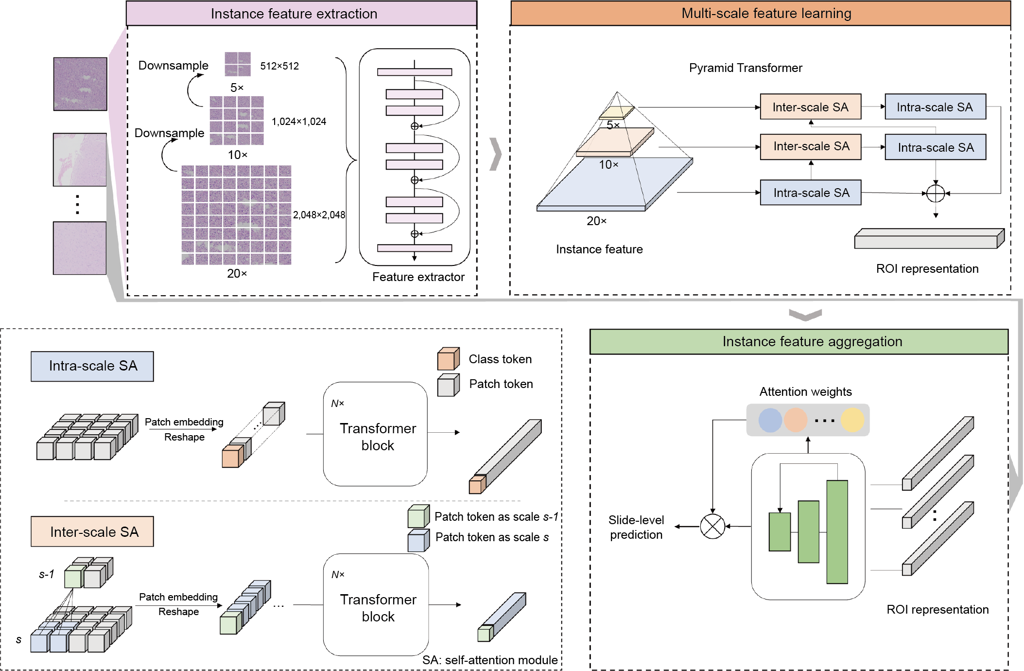
A transformer-based weakly supervised computational pathology method for clinical-grade diagnosis and molecular state revelation of gliomas
Python (3.8.13), h5py (3.6.0), openslide (version 3.4.1), opencv (version 4.5.5), pillow (version 6.2.1), Pytorch (version 1.12.1), scikit-learn (version 1.0.2), matplotlib (version 3.5.2) and seaborn (version 0.11.2).
We recommend that you use anaconda to configure ROAM’s dependency environment. You can refer to https://www.anaconda.com/distribution/ to download and install the anaconda corresponding to the python version you are using.
Use the environment configuration file located in ./docs/environment.yaml to create a conda environment:
conda env create -n roam -f docs/environment.yamlActivate the roam environment to run the training code:
conda activate roamIf an error occurs when importing h5py, you can try uninstalling and then reinstalling the package.
pip uninstall h5py
pip install --no-cache-dir h5pyWe provide the complete process of using ROAM. You can modify related config files and parameters to train ROAM with your own dataset. We provide slide example and trained models for reproducibility. The detailed information can be found in slide examples and model checkpoints.
The first step is to prepare training dataset. The WSI data should be first segmented to several patches (ROI in ROAM, size is
WSI data and corresponding detailed information (.csv file) shoule be ready. The format of digitized whole slide image data should be standard formats (.svs,.tiff etc.) that can be read with openslide (version 3.4.1).
Here is an example of directory for WSI data.
DATA_DIRECTORY
      |____ slide1.tiff
      |____ slide2.tiff
      |____ ...
The corresponding information data of WSI (.csv) should include key information such as slide_id,path,label. Here is an example:
| slide_id | path | label | level |
|---|---|---|---|
| 965c821d05bbec8 | /images/202007/965c821d05bbec8.tif | 2 | 20x |
level is the magnification level of the slide. More information can be added to facilitate the process of the data. We provide an example csv file in ./data_prepare/data_csv/.
The first step is to segment the tissue and crop patches from the tissue region. We referenced CLAM's WSI processing method. CLAM provide a robust WSI segmentation and patching implementation. You can refer to CLAM for more detailed information.
You can segment the tissue region and crop patches by running the following command in ./data_prepare/ directory:
python create_patches_fp.py --source DATA_DIRECTORY --datainfo DATA_INFO_DIRECTORY --patch_size 4096 --step_size 4096 --save_dir PATCH_DIRECTORY --patch_level 0 --seg --stitch --patchThe description of parameters is listed as follow:
--source:path to raw wsi data
--datainfo: data information of WSI data
--patch_size: size of patch
--step_size: step size of patching, "patch_size == step_size" denotes patches are extracted without overlapping
--save_dir: path to save results
--patch_level: downsample level at which to crop patches
--seg,--stitch,--patch: Indicate whether to split the slides, whether to concatenate the segmengted patches to observe the segmentation effect, and whether to extract patches.
The above commond will segment all WSIs in DATA_INFO_DIRECTORY (.csv file), crop patches within the tissue regions with the size of 2048 and generate the following folder structure:
PATCH_DIRECTORY
      |____ masks
            |__ slide1.jpg
            |__ slide2.jpg
            |__ ...
      |____ patches
            |__ slide1.h5
            |__ slide2.h5
            |__ ...
      |____ stitches
            |__ slide1.jpg
            |__ slide2.jpg
            |__ ...
      |____ process_list_autogen.csv
The masks folder contains the segmentation results (one image per slide).
The patches folder contains arrays of extracted tissue patches from each slide (one .h5 file per slide, where each entry corresponds to the coordinates of the top-left corner of a patch)
The stitches folder contains downsampled visualizations of stitched tissue patches (one image per slide)
Please note that the slide example we provide was obtained at a magnification level of 40x. The actual size of the ROI extracted is
When utilizing your own dataset, remember to guarantee that the size of extracted ROI is
For each ROI (patch with size of
Run the following commond in ./data_prepare/ directory for feature extraction:
python extract_feature_patch.py --data_h5_dir PATCH_DIRECTORY --data_slide_dir DATA_DIRECTORY --csv_path DATA_INFO_DIRECTORY --feat_dir FEAT_DIRECTORY --pretrained_model ImageNet --is_stain_normParameters:
--feat_dir: directory to save features results.
--pretrained_model: pre-trained model to extract patch features. "ImageNet","RetCCL","ctranspath","simclr-ciga" are available models. "ImageNet" denotes ResNet50 pretrained with ImageNet. Other 3 models are self-supervised models for pathological images. You can refer to RetCCL, ctranspath, simclr-ciga for model checkpoint and detailed information.
--is_stain_norm: whether to use stain normalization
The above commond will generate features with following folder structure:
FEAT_DIRECTORY
      |____ feats_ImageNet_norm
            |__ slide1.h5
            |__ slide2.h5
            |__ ...
Each .h5 file contains an array of extracted features and corresponding coordinates. Features shape of each ROI is
We provide some model codes that may be needed for feature extraction in ``data_prepare/models/`, including "ImageNet","RetCCL","simclr-ciga", etc. The corresponding checkpoint files can be downloader from pretrained model weights.
ROAM employs a 5-fold cross validation on the training dataset, followed by testing the ensemble of the 5 trained models on the test dataset. The format of splits data is .npy file. The file contains the training and validation set splits for each fold.
Each fold contains train list, train labels, val list and val labels:
## fold 1
(
      [train_slide_id1,train_slide_id2,...,train_slide_idk],
      [train_label1,train_label2,...,train_labelk],
      [val_slide_id1,val_slide_id2,...,train_slide_idm],
      [val_label1,val_label2,...,val_labelm]
)
## fold 2
...
For test split, the format of split data is:
np.array([
      [test_slide_id1,test_slide_id2,...,test_slide_idk],
      [test_label1,test_label2,...,test_labelk]
])
We provide examples of splits in ./data_prepare/data_split/
With features data and splits, you can start training your own ROAM models.
You should first prepare config file and script file. You can easily modify the parameters in config files and then list training commond in script file. Run the script file to train ROAM models. It can effectively standardizes the code training, avoiding the need to input lengthy training commands.
config file (.ini file) is created in the ./ROAM/configs folder. Here we list some of the main parameters. For more detailed settings, please refer to ./ROAM/parse_config.py:
[int_glioma_tumor_subtyping] #task

seed=1 #initial random seed for traininng
stage=train #train or test
embed_type=ImageNet #pre-trained model that features are extracted
not_stain_norm=False #whether to use stain-noramlized features
data_root_dir=../data_prepare/FEAT_DIRECTORY #directory of features
results_dir=RESULT_DIRECTORY #directory to save final results
...
About 'data_root_dir': Please note that codes for model training and feature extraction aren't executed under the same
root directory. Feature extraction is in data_prepare, and training is in ROAM. Therefore, providing the relative path
to the original extracted feature (FEAT_DIRECTORY) would cause an error. You can either use absolute paths or prepend ../data_prepare to the path.
For example, we set FEAT_DIRECTORY=./example, then data_root_dir should be ../data_prepare/example.
You can define your own task in ./ROAM/parse_config.py. Here is an example of task in our experiments:
task_info={
      'int_glioma_tumor_subtyping':{
            'csv_path': DATA_INFO_DIRECTORY,
            'label_dict': {0:0,1:1,2:2,3:2,4:2}, # map the original labels to the labels required for this task
            'n_classes': 3, # number of classes
            'split_dir': '../data_prepare/data_split/xiangya_split_subtype/example_int_glioma_tumor_subtyping.npy', # training splits
            'test_split_dir':  '../data_prepare/data_split/xiangya_split_subtype/example_test_split.npy', # test splits
            'cls_weights': [50,24,514], # the proportion of each class in the training dataset, for class balance when generating dataloader.
      }
}
We also provide examples for reference: ./ROAM/configs/int_glioma_tumor_subtyping.ini. Please note that the parameters in the config file must be defined in parse_config.py.
script file (.sh file) is created in ./ROAM/scripts folder. You need only provide config file, splits seed and experiment name (can be omitted). Here is an example of ./ROAM/scripts/int_glioma_tumor_subtyping.sh:
cd ..
python main.py configs/int_glioma_tumor_subtyping.ini s1 example1
python main.py configs/int_glioma_tumor_subtyping.ini s2 example2
The script indicates that we conduct 2 experiments using 2 different splits seed. The split seed refers to the random seed number used for dividing the training and val splits. We conducted five experiments with different split seeds (denoted as s0 to s4) to enhance the robustness and credibility of the experimental results in the paper.
training
With config file and script file, you can train ROAM models with following commond in ./ROAM/scripts/ directory:
CUDA_VISIBLE_DEVICES=0 sh int_glioma_tumor_subtyping.shResults directory
The code will automatically save the best-performing model and evaluation metrics for each fold during the training process.
The results will be saved in {result_dir}/{task}/{exp_code}/{seed}.
results_dir is the root directory to save results.
task is the task name of the experiment. For example, we provide a example task "int_glioma_tumor_subtyping".
seed is the random seed of this experiment. These three parameters can be configured in the config file. You can refer to ./ROAM/configs/int_glioma_tumor_subtyping.ini
exp_code is the code name of this experiment. You can either customize it or use the default name. You can set "exp_code" in training script file. For example, we provide a example script file: scripts/int_glioma_tumor_subtyping.sh:
python main.py configs/int_glioma_tumor_subtyping.ini s1 exp_code #you can remove the exp_code to use the default settingThe details of default "exp_code" can be found in parse_config.py:
args.exp_code = '_'.join(map(str, [args.task, args.depths,
                                       args.embed_type,
                                       args.batch_size, args.roi_dropout,
                                       args.roi_supervise,
                                       args.roi_weight, args.topk,
                                       args.roi_level,
                                       args.scale_type,args.single_level,
                                       args.not_interscale]))
Here we provide an example folder structure of saved results:
results
      |____ int_glioma_tumor_subtyping
            |____ int_glioma_tumor_subtyping_[2, 2, 2, 2, 2]_ImageNet_4_True_True_1.0_4_0_ms_0_False
                  |____ s1
                        |____ visual_res
                              |__ cm_mean.png # confusion matrix on test dataset
                              |__ normal_cm_mean.png
                              |__ metrics.json # resutls summary
                        |____ ROAM_split0.pth #model checkpoints for each fold
                        |____ ROAM_split1.pth
                        |____ ROAM_split2.pth
                        |____ ROAM_split3.pth
                        |____ ROAM_split4.pth
                        |____ results.json #complete results, including probs,preds,... of each fold
If you want to run the testing and visualization code using the example model weights we provide, please download the five model weights and place them according to the folder structure outlined above.
test
You can also test the model performance with following commond:
CUDA_VISIBLE_DEVICES=0 sh int_glioma_tumor_subtyping_test.shConfigure file is the same as the configure file in the training section. Here is an example of the script for cascade diagnosis:
cd ..
python predict_cascade.py configs/int_glioma_cls.ini s1 #for glioma detection
python predict_cascade.py configs/int_glioma_tumor_subtyping.ini s1 #for glioma subtyping
python predict_cascade.py configs/int_ast_grade.ini s1 #for astrocytoma grading
python predict_cascade.py configs/int_oli_grade.ini s1 #for oligodendroglioma grading
python predict_cascade.py configs/int_epe_grade.ini s1 #for ependymoma grading
The results will be saved in ./ROAM/prediction_results/ by default.
Then run the script to generate the complete diagnosis resutls in ./ROAM/scripts/:
CUDA_VISIBLE_DEVICES=0 sh cascade_pred.shWe provide an example of the script for predicting the subtype of the slides: ./ROAM/scripts/cascade_pred_int_glioma_tumor_subtyping.sh
You can also try ablation experiments to validate ROAM's performance in ./ROAM/ablations.
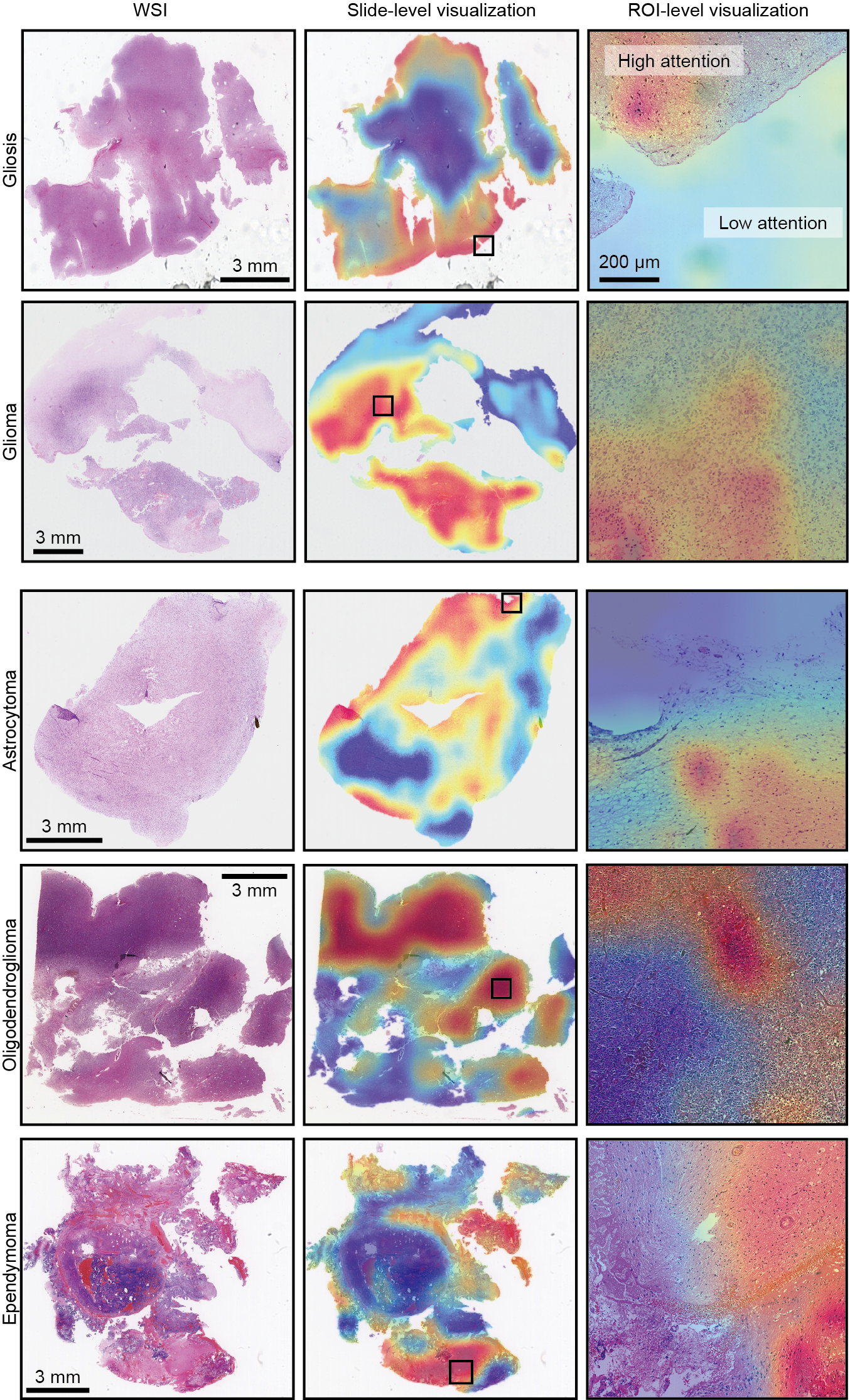
We provide both slide-level and roi-level visualization methods.
slide-level visualization
We generate WSI attention heatmap using attention score of each roi. Config file and visualization results are saved in ./ROAM/visheatmaps/slide_vis.
Run the following commond to generate slide-level visualization results:
python gen_visheatmaps_slide_batch.py config_int_glioma_tumor_subtyping.yaml s1config file should be in ./ROAM/visheatmaps/slide_vis/configs/ and 's1' is split seed.
Please note that you need to modify the path of the slide image in the ./ROAM/visheatmaps/slide_vis/process_list/int_glioma_tumor_subtyping.csv, keeping the path consistent with DATA_DIRECYOTY in WSI segmentation and patching.
roi-level visualization
ROI-level visualization is performed through calculate gradients of patch tokens in the self-attention matrix. For more detailed information you can refer to Transformer-Explainability and vision-transformer-explainability. Config file and visualization results are saved in ./ROAM/visheatmaps/roi_vis.
Run the following commond to generate roi-level visualization resutls:
python gen_visheatmaps_roi_batch.py visheatmaps/roi_vis/configs/int_glioma_tumor_subtyping_vis_roi.ini s1For reproducability, we provide a oligodendroglioma slide example and its corresponding feature extracted from ImageNet pretrained ResNet50. The slide and feature can be downloaded from: slide examples
With its corresponding test split:
./data_prepare/data_split/xiangya_split_subtype/example_test_split.npy
data infomation:
./data_prepare/data_csv/example_xiangya_data_info_pro.csv
and configure, script file, you can test the ROAM model with the example slide.
For reproducability, we provide 5 trained models with 5 different split seeds for glioma subtyping task.
Model checkpoints: model_ckpt
Here are some examples of visualization results.
- Add the pretrained model codes in
data_prepare/modelsand provide the corresponding checkpoints. - Add another 2 dependencies: spams(version 2.6.5.4) and torchsummary(version 1.5.1).
- Update the command of WSI segmentation and patching.
- Add a description for the saving path of the training results in training and test section.
- Fix a bug where the feature paths during model prediction is inconsistent with the previously generated paths.
- Fix a potential bug in "predict_cascade.py" during prediction.
- Update the figure of framework
- Fix some typos.
If you find our work helpful for your research, please consider citing our article:
Jiang, R., Yin, X., Yang, P. et al. A transformer-based weakly supervised computational pathology method for clinical-grade diagnosis and molecular marker discovery of gliomas. Nat Mach Intell (2024). https://doi.org/10.1038/s42256-024-00868-w


