ARFIMA.jl

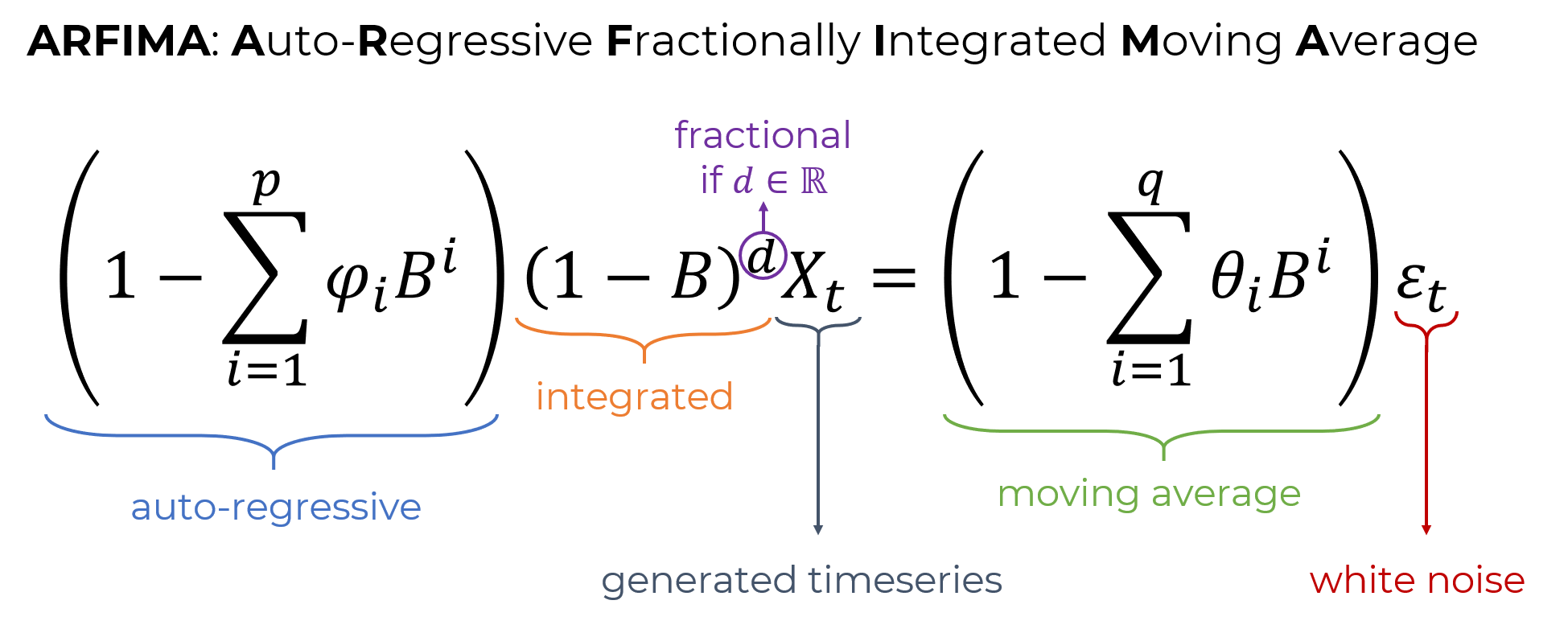
This Julia package simulates stochastic timeseries that follow the ARFIMA process, or any of its simplifications: ARIMA/ARMA/AR/MA/IMA.

The code base is also a proof-of-concept of using Julia's multiple dispatch.

This package is unregistered (because of the absence of a test suite). To install do:

julia> ] add https://github.com/JuliaDynamics/ARFIMA.jl

julia> using ARFIMA

see the examples below for usage.

ARFIMA and its variants

The ARFIMA process is composed out of several components and each can be included or not included in the process, resulting in simplified versions like ARMA.

Usage

This package exports a single function arfima. This function generates the timeseries Xₜ using Julia's multiple dispatch.

Here is its documentation string:

arfima([rng,] N, σ, d, φ=nothing, θ=nothing) -> Xₜ

Create a stochastic timeseries of length N that follows the ARFIMA process, or any of its subclasses, like e.g. ARMA, AR, ARIMA, etc., see below. σ is the standard deviation of the white noise used to generate the process. The first optional argument is an AbstractRNG, a random number generator to establish reproducibility.

Julia's multiple dispatch system decides which will be the simulated variant of the process, based on the types of d, φ, θ.

Variants

The ARFIMA parameters are (p, d, q) with p = length(φ) and q = length(θ), with p, q describing the autoregressive or moving average "orders" while d is the differencing "order". Both φ, θ can be of two types: Nothing or SVector. If they are Nothing the corresponding components of autoregressive (φ) and moving average (θ) are not done. Otherwise, the static vectors simply contain their values.

If d is Nothing, then the differencing (integrated) part is not done and the process is in fact AR/MA/ARMA. If d is of type Int, then the simulated process is in fact ARIMA, while if d is AbstractFloat then the process is ARFIMA. In the last case it must hold that d ∈ (-0.5, 0.5). If all d, φ, θ are nothing, white noise is returned.

The function arma(N, σ, φ, θ = nothing) is provided for convienience.

Examples

N, σ = 10_000, 0.5
X = arfima(N, σ, 0.4)                             # ARFIMA(0,d,0)
X = arfima(N, σ, 0.4, SVector(0.8, 1.2))          # ARFIMA(2,d,0)
X = arfima(N, σ, 1, SVector(0.8))                 # ARIMA(1,d,0)
X = arfima(N, σ, 1, SVector(0.8), SVector(1.2))   # ARIMA(1,d,1)
X = arfima(N, σ, 0.4, SVector(0.8), SVector(1.2)) # ARFIMA(1,d,1)
X = arfima(N, σ, nothing, SVector(0.8))           # ARFIMA(1,0,0) ≡ AR(1)

Benchmarks

Some benchmark code is included in src/benchmarks.jl. These results come from running the code on a laptop with Windows 10, Julia 1.2.0, Intel i5-6200U @2.30GHz CPU, 8192MB RAM. Results that need microseconds to run are not timed accurately.

Process: ARFIMA(0, d=0.4, 0)
For N = 10000, 0.2449999 seconds
For N = 50000, 1.467 seconds
For N = 100000, 7.5779998 seconds

Process: ARIMA(0, d=2, 0)
For N = 10000, 0.0 seconds
For N = 50000, 0.0009999 seconds
For N = 100000, 0.0020001 seconds

Process: ARFIMA(φ=0.8, d=0.4, 0)
For N = 10000, 0.267 seconds
For N = 50000, 1.388 seconds
For N = 100000, 7.4589999 seconds

Process: ARMA(φ=0.8, θ=2.0)
For N = 10000, 0.0 seconds
For N = 50000, 0.0009999 seconds
For N = 100000, 0.003 seconds

Acknowledgements

Thanks to Katjia Polotzek for providing an initial code base for ARFIMA and to Philipp Meyer for validation of parts of the code