William R.P. Denault 26/02/2021
A complete CFMR pipeline with random splits is provided in the folder CFMR_pipeline_code.
Here we present basic scripts to obtain a cross-fitted instrument. For the sake of simplicity, we don’t partition the data at random.
Here we define the parameters of our analysis
# n number of individuals
n <- 3000
# p  Number of selected SNPs
p <- 100
# np_act Number of SNPs affecting the exposure among the p selected SNPs
np_act <-5
# sub_split Number of splits
sub_split <- 5
Below we simulate the data. G contains the selected SNPs (p) and the (np_act) first columns of G contain the actual causal SNPs. X and Y are sampled with correlated noise (0.7) and H is the hidden confounded
set.seed(1)
#Y and X are sample with some correlated noise
noise <-rmvnorm(n, mean = rep(0, 2), sigma = matrix(nrow = 2,
                                                    byrow = TRUE,
                                                    c(1,0.7,0.7,1)
                                                    )
                )
#Genotype data, each of the SNP are sample at Hardy-Weinberg equilibrium for a MAF of 30%
  G <- matrix(sample(c(0,1,2),
                     size= (n*p),
                     prob = c(0.7^2, 2*0.7*0.3, 0.3^2),
                     replace = TRUE),
              nrow= n)
#Hidden confounding, increase sd to increase confounding
H <- rnorm(n, sd=1)

#ZPI is the part of X explained by the SNPs
ZPI <- 0.5*apply( G[, (1:np_act)],1, mean )

#X is compound of ZPI, H hidden confounding, and a noise that correlates with the noise of Y
X <- ZPI+H+ noise[,2]
#Y the exposure also affected by H
Y <- X+H+noise[,1] #Effect of X on Y is 1
cor(H,X)
## [1] 0.6932508
cor(H,Y) # large confouding## [1] 0.7237769
plot(X,Y,
     main="Bivariate plot of X and Y")

res0 <- lm(Y~X)
abline(a=0,b=summary(res0)$coef[2,1], col="blue", lwd=2)
abline(a=0,b=1, col="green", lwd=4, lty=2)
legend( x=-5, y=7,
        bty = "n",
        lty= c(1,1,1,2),
        legend=c("Confouded estimate" , "Truth"),
        col= c("blue","green"),
        lwd=rep(2,4))
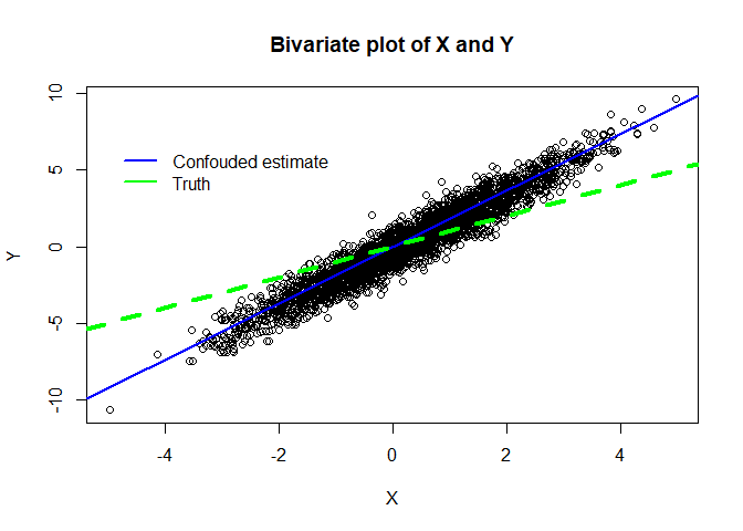
The plot above shows the observational association (blue line) between X and Y. It is is heavily confounded by the hidden confounder H as the correlation between H and X is 0.69, and the correlation between H and Y is 0.72. The blue dashed line represent the true effect of X on Y.
Below the function used to obtain a cross-fitted instrument
#function to perform the cross fitting
build_IV_sub_sample <- function(i) #i in 0:(sub_split-1)
{
  indx <- (1+i*(n/sub_split)):((i+1)*(n/sub_split))# here the splits are not random
  Gtemp <- G[-indx,]
  Xtemp <- X[-indx]
  lasso <-  cv.glmnet(x=Gtemp, y=Xtemp,alpha=1)
  return(predict(lasso, G[indx,], s = "lambda.min")
  )
}
Here we estimate the effect of X on Y using three approaches, a naive linear model, a one-sample instrument based on LASSO, and a cross-fitted instrument based on LASSO.
###Standard linear model
res0 <- lm(Y~X)

#Identification and estimation of the insturement within the sample
lasso <-  cv.glmnet(x=G,y=X,alpha=1)

IV <-  predict(lasso,G,s = "lambda.min")
res1 <- ivreg(Y~X|IV)

# CFI estimation
res  <- lapply(0:(sub_split-1), build_IV_sub_sample)#performing cross-fitting
CFI <- do.call(c,res)
#cross fitted IV, CFMR2
res2 <- ivreg(Y~X|CFI)


plot(X,Y, main="Estimation of the effect of X on Y")
abline(a=0,b=summary(res0)$coef[2,1], col="blue", lwd=2)
abline(a=0,b=summary(res1)$coef[2,1], col="red", lwd=2)
abline(a=0,b=summary(res2)$coef[2,1], col="springgreen4", lwd=2)
abline(a=0,b=1, col="green", lwd=4, lty=2)
legend( x=-5, y=7,
        bty = "n",
        lty= c(1,1,1,2),
        legend=c("Linear model", "One sample instrument LASSO","CFI with LASSO" , "Truth"),
        col= c("blue", "red","springgreen4", "green"),
        lwd=rep(2,4))
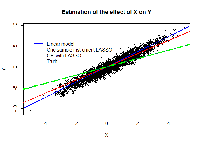
The plot above shows the estimates of the effect of X on Y using different appraoches. CFI with LASSO (solid green line) is the closest to the true effect of X on Y. One sample instrument with LASSO (solid red line) is biased towards the confounded estimate based on linear model (solid blue line).
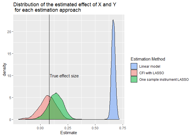
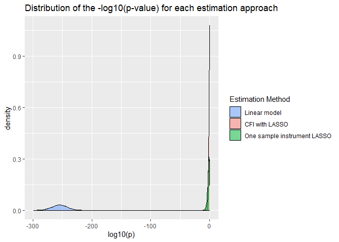
Here we simulate 3000 data sets and on each of them wethe effect of X on Y (simulation parameters n=2000, p=100, np_act=5,beta=0.08,h2=0.1) using CFI, one sample instrument LASSO estimate, and a standard linear model. The function used for the simulations can be found at the end of this document or in the folder CFMR_simulation_code.
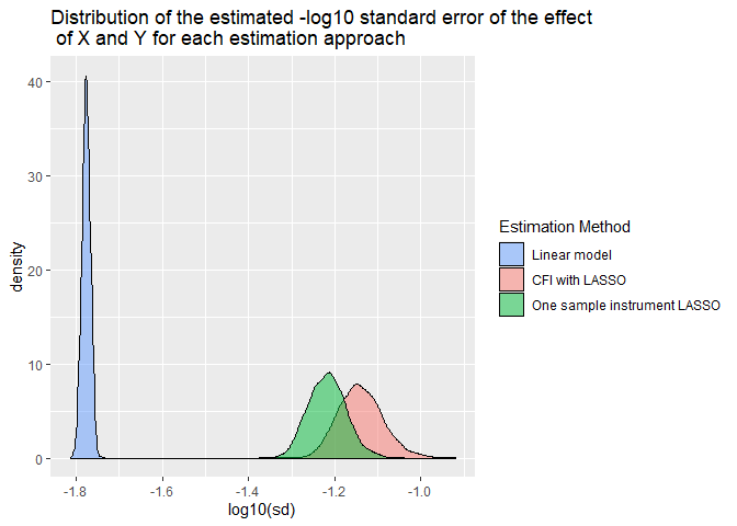
Clearly, LM and one sample IV Lasso are overconfident and biased. In the plot below, we see that the linear model and On sample instrument LASSO have smaller standard errors than CFI with LASSO, which implies overconfidence in the significance of the estimated effect.
#n integer sample size of the analysis
#p number of selected SNP
#np_act number of SNPs actually modifying the exposure among the p selected SNP.
#h2 exposure variance explained by the np_act SNPs
#beta effect size of the exposure on the outcome

simu_cross_fit_IV_est <- function(n,p,np_act, h2, beta )
{
  if( missing(h2))
  {
    h2 <- 0.2
  }

  if( missing(beta))
  {
    beta <- 1
  }
  if(np_act >p)
  {
    print( "np_act should be smaller than p")
    break
  }
  n <- n
  #Number of selected SNPs
  p <- p
  #Number of SNPs affecting the exposure
  np_act <- np_act
  #Genotype data
  G <- matrix(sample(c(0,1,2),
                     size= (n*p),
                     prob = c(0.7^2, 2*0.7*0.3, 0.3^2),
                     replace = TRUE),
              nrow= n)

  #Y and X are sample with some correlated noise
  noise <-rmvnorm(n,
                  mean = rep(0, 2),
                  sigma = matrix(nrow = 2,
                                 byrow = TRUE,
                                 c(1,0.7,0.7,1)
                  )
  )


  V <- noise[,2]

  U <- noise[,1]


  #rescaling for insuring h2 = h2 on average
  tt <- apply( G[, (1:np_act)],1,sum)#genotype effect
  if( h2==0)
  {
    resc <- 0
  }else{resc <- ((var(H)+var(V))*(h2/(1-h2)))/var(tt)


  }

  ZPI <- sqrt(resc)*tt


  #X is compound of ZPI , H hidden confounding, and a noise that correlates with the noise of Y

  X <- ZPI + H + V

  #Y the exposure also affected by H

  Y <- beta*X + H + U

  build_IV_sub_sample <- function(i)
  {
    indx <- (1+i*(n/sub_split)):((i+1)*(n/sub_split))


    Gtemp <- G[-indx,]
    Xtemp <- X[-indx]

    lasso <-  cv.glmnet(x=Gtemp, y=Xtemp,alpha=1)
    return(predict(lasso, G[indx,], s = "lambda.min"))
  }


  #LM estimate
  res1 <- summary(lm(Y~X))$coef[2,]
  #Cross fitting LASSO
  res  <- lapply(0:(sub_split-1), build_IV_sub_sample)
  IV   <- do.call(c,res)
  res2 <- summary(ivreg(Y~X|IV))$coef[2,]

  #One sample lasso IV
  lasso <-  cv.glmnet(x=G, y=X,alpha=1)
  IV <- predict(lasso, G, s = "lambda.min")
  res3 <- summary(ivreg(Y~X|IV))$coef[2,]


  out  <- data.frame(rbind(res1,res2,res3))
  out$type <- c("LM","CFI_LASSO","IV_LASSO")

  return(out)
}