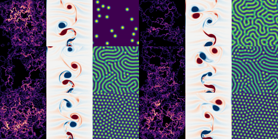
(Left to Right): Avalanche activity cascades in a sandpile automaton; a vortex street formed by flow past a cylinder; and Turing patterns in a reaction-diffusion model. All simulations from the course homeworks; a higher-resolution video may be viewed here
Materials for computational physics course, taught by William Gilpin.
This course aims to provide a very broad survey of computational methods that are particularly relevant to modern physics research. We will aim to cover efficient algorithm design and performance analysis, traditional numerical recipes such as integration and matrix manipulation, and emerging methods in data analysis and machine learning. Our goal by the end of the class will be to feel comfortable approaching diverse, open-ended computational problems that arise during research, and to be ready to design and share new algorithms with the broader research community.
The class website is located here.
- If you are enrolled in 329 at UT, the syllabus and calendar are here.
- If you are enrolled in 381C at UT, the syllabus and calendar are here.
- For both UT courses, the Discussions page may be found here.
Many links below direct to Google Colab, and can be run-in-browser without installation as long as you are signed into a Google account. To download the raw source files, please refer to the GitHub repository. Some lecture videos are linked below, and the remaining lecture videos are linked in the Syllabus (above).
- HW1: The sandpile cellular automaton and directed percolation. [ipynb] Covers recursion, runtime scaling, vectorization
- HW2: Linear dynamical systems and decomposing a chaotic flow. [ipynb] Covers numerical linear algebra, optimization, and unsupervised learning
- HW3: Turing patterns and phase separation. [ipynb] Covers numerical integration; finite-differences and spectral methods
- HW4: Predicting turbulence with operator methods. [ipynb] Covers Supervised learning, time series forecasting, ridge, kernel, and logistic regression
-
Lecture 1: Python syntax for Scientific Computing
[html] [ipynb] -
Lecture 2: Object-oriented programming to find first-passage times of Brownian motion
[html] [ipynb]
-
Lecture 5: Finding the Feigenbaum constant with recursion and dynamic programming
[html] [ipynb] -
Lecture 6: Detecting the onset of turbulence with the Fast Fourier Transform
[html] [ipynb]
-
Lecture 9: Probing social networks with PageRank
[html] [ipynb] -
Lecture 10: Spectral graph theory and the QR eigenvalue algorithm
[html] [ipynb]
-
Lecture 12: Krylov subspace methods & Conjugate gradient methods
[html] [ipynb] -
Lecture 15: Multivariate Optimization and Potential Flows
[html] [ipynb]
-
Lecture 16: Evolving Cellular Automata with Genetic Algorithms
[html] [ipynb] -
Lecture 17: Monte Carlo methods and Hard Sphere Packing
[html] [ipynb] -
Lecture 18: Numerical Integration and predicting chaos
[html] [ipynb]
-
Lecture 21: Diffusion, relaxation, and instability
[html] [ipynb] -
Lecture 22: Shocks, solitons, and hyperbolic partial differential equations
[html] [ipynb]
-
Lecture 24b: Supervised Learning of cellular automaton dynamics
[html] [ipynb] -
Lecture 25: Classification, Logistic Regression, and phases of matter
-
Lecture 26: Overfitting, bias-variance tradeoff, and double-descent
[html] [ipynb] -
Lecture 28: Time series representation, featurizing chaos, kernel methods
[html] [ipynb] -
Lecture 29: Gaussian mixtures, expectation-maximization, and superresolution microscopy
[html] [ipynb] -
Lecture 30: Predicting the Reynolds number of turbulence with deep learning
[html] [ipynb]
-
Lecture 31: Types of neural networks; symmetries in physical systems
[html] [ipynb] -
Lecture 32: Training neural networks with backpropagation
[html] [ipynb] -
Lecture 33: Reservoir computers and forecasting chaotic systems
[html] [ipynb]
- How to use the high-performance computing cluster
- Matrix Derivatives notes
- Hopfield Networks and Spin Glasses [ipynb]
- Variational Autoencoders [ipynb]
- Vector-Quantized Variational Autoencoders (VQ-VAE) [ipynb]
- Lab 1: Getting started with Python
- Lab 2: git, GitHub, and GitHub Pages
- Lab 3: Documentation and Formatting
- Lab 4: Automatically creating online documentation with Sphinx
- Lab 5: Unit Testing
- Lab 6: Structuring an Open-Source Repository
The guidelines and rubric for the final project and presentation can be found here
- Quantum Reinforcement Learning with the Grover method
- Modelling the contractile dynamics of muscle
- Tight binding and Anderson localization on complex graphs
- Neural System Identification by Training Recurrent Neural Networks
- Assimilating a realistic neuron model onto a reduced-order model
- Testing particle phenomenology beyond the Standard Model with Bayesian classification
- Monte Carlo sampling for many-body systems
If you are teaching a similar course, please feel free to use any or all of these materials. If you have any suggestions for improvements or find any errors, I would very much appreciate any feedback. Consider submitting corrections as issues or pull requests on GitHub.
For students, logistics and project questions are best posted on the classroom forum (Ed Discussions); errors in the materials should be issues on the course repository; for other issues, I can be reached via email
We will primarily use Python 3 with the following packages
- numpy
- matplotlib
- scipy
- scikit-learn
- jupyter
For projects and other parts of the class, you might also need
- ipykernel
- scikit-image
- umap-learn
- statsmodels
- pytorch
- jax
- numba
Portions of the material in this course are adapted or inspired by other open-source classes, including: Pankaj Mehta's Machine Learning for Physics Course, Chris Rycroft's Numerical Recipe's Course, Volodymyr Kuleshov's Applied Machine Learning course, Fei-Fei Li's Deep Learning for Computer Vision course, Lorena Barba's CFD course and Jim Crutchfield's Nonlinear Dynamics course
<script async src="https://www.googletagmanager.com/gtag/js?id=G-37RSFCXBQY"></script> <script> window.dataLayer = window.dataLayer || []; function gtag(){dataLayer.push(arguments);} gtag('js', new Date()); gtag('config', 'G-37RSFCXBQY'); </script>