willtai/ad_examples

A collection of popular anomaly detection methods (iid/point-based and time series) including active learning for anomaly detection/discovery, description for diversity/explanation/interpretability. With a deeper analysis of incorporating label feedback with ensemble and tree-based detectors. Includes results-plots and illustrations for most approaches covered.

Python libraries required:

numpy (1.14.2)
scipy (1.0.0)
scikit-learn (0.19.1)
cvxopt (1.1.9)
pandas (0.21.0)
ranking (0.3.1)
statsmodels (0.8.0)
matplotlib (2.1.0)
tensorflow (1.6.0)

Note: The code has been tested with python 2.7.

Anomaly Detection Examples

This is a collection of anomaly detection examples for detection methods popular in academic literature and in practice. I will include more examples as and when I find time.

Some techniques covered are listed below. These are a mere drop in the ocean of all anomaly detectors and are only meant to highlight some broad categories. Apologies if your favorite one is currently not included -- hopefully in time...

• i.i.d setting:
  • Standard unsupervised anomaly detectors (Isolation Forest, LODA, One-class SVM, LOF)
  • Clustering and density-based
  • Density estimation based
  • PCA Reconstruction-based
  • Autoencoder Reconstruction-based
  • Classifier and pseudo-anomaly based
  • Ensemble/Projection-based
  • A demonstration of outlier influence
  • Spectral-based
• timeseries
  • Forecasting-based
    • ARIMA
    • Regression (SVM, Random Forest, Neural Network)
    • Recurrent Neural Networks
  • i.i.d
    • Windows/Shingle based (Isolation Forest, One-class SVM, LOF, Autoencoder)
• human-in-the-loop (active learning)
  • Active Anomaly Discovery (batch setup, streaming setup) -- Includes plots and illustrations (see sections below)
    • High-level summary of the approach
    • Jump right in: General instructions on running AAD
    • Explanations and Interpretability: Generating anomaly descriptions with tree-based ensembles
    • Query strategies: Diversifying query instances using the descriptions and its evaluation
    • Some properties of different tree-based detectors
    • Running AAD with precomputed ensemble scores
    • Data drift detection and model update with streaming data
    • A bit of theoretical intuition
• Reducing activity sequences to i.i.d -- This illustrates an approach that is becoming increasingly popular as a starting-point for anomaly detection on activity sequences and transfer learning.

There are multiple datasets (synthetic/real) supported. Change the code to work with whichever dataset or algorithm is desired. Most of the demos will output pdf plots under the 'python/temp' folder when executed.

AUC is the most common metric used to report anomaly detection performance. See here for a complete example with standard datasets.

To execute the code:

1. Run code from 'python' folder. The outputs will be generated under 'temp' folder. The pythonw command is used on OSX, but python should be used on Linux.

2. To avoid import errors, make sure that PYTHONPATH is configured correctly to include the current dir: .:/usr/local/lib/python

3. The run commands are at the top of the python source code files.

4. Check the log file in python/temp folder. Usually it will be named <demo_code>.log. Timeseries demos will output logs under the python/temp/timeseries folder.

Active Anomaly Discovery (AAD)

This codebase replaces the older 'pyaad' project (https://github.com/shubhomoydas/pyaad). It implements an algorithm (AAD) to actively explore anomalies.

The main idea that helps understand AAD can be summarized as follows:

• Uncertainty sampling for active learning in standard classification setting is label efficient
• Anomaly detector ensembles, by design, enable uncertainty sampling for anomaly detection (this is not obvious) such that both learning the margin (in a linear model) as well as discovering anomalies is efficient:
  • For uncertainty sampling with a linear model, the hyperplane margin should pass through the region of uncertainty
  • The uncertainty region has a well-known prior when anomaly detector ensembles are employed
  • AAD designs a hyperplane that passes through the uncertainty region and tries to maintain it there so that uncertainty sampling can then be employed for anomaly detection
  • instances on one side of the margin are much more likely to be anomalies than on the other side; presenting instances from the 'anomaly' side to the analyst then reveals true anomalies faster

The desired properties of an ensemble-based detector which will make it well-suited for active learning are:

• Inexpensive members: computationally cheap to create ensemble members. If we employ a linear model (such as with AAD), it helps to have a large number of members because it then increases the capacity of the model to incorporate a large number of instance labels.
• Somewhat-OK (weak?) accuracy: if accuracy is low, then more members will be desired
• Many and diverse members: a large number of high-precision-low-recall members might work well in combination (such as the leaf nodes of tree-based detectors)

Some anomaly detectors which fit the above desiderata are:

• LODA: The one-dimensional projections are the members
• Tree-based detectors such as Isolation Forest: We may treat each tree in the forest or each node in the trees as the members
• Feature bagging: Detectors created from each random feature subset act as the members

The section 'Intuition behind Active Anomaly Discovery' below explains the idea in more depth.

Assuming that the ensemble scores have already been computed, the demo code percept.py implements AAD in a much more simplified manner.

To run percept.py:

pythonw -m percept.percept

The above command will generate a pdf file with plots illustrating how the data was actively labeled.

Reference(s):

• Das, S., Wong, W-K., Dietterich, T., Fern, A. and Emmott, A. (2016). Incorporating Expert Feedback into Active Anomaly Discovery in the Proceedings of the IEEE International Conference on Data Mining. (pdf)(presentation)

• Das, S., Wong, W-K., Fern, A., Dietterich, T. and Siddiqui, A. (2017). Incorporating Feedback into Tree-based Anomaly Detection, KDD Interactive Data Exploration and Analytics (IDEA) Workshop. (pdf)(presentation)

• Das, S. (2017). Incorporating User Feedback into Machine Learning Systems, PhD Thesis (pdf) -- Much of the work on AAD in this repository originated during my PhD research.

Running AAD

This codebase is my research platform. The main bash script aad.sh makes it easier to run all AAD experiments multiple times (in the spirit of scientific inquiry) so that final results can be averaged. I try to output results for different parameter settings into different folders (under python/temp/aad) so that results can be easily compared without conflicts. I also output to files the instance indexes (as 1-indexed and not 0-indexed) in the order they were queried for fine-grained analysis and visualization. If you want to introduce a new dataset with the least effort, then put its files under datasets/anomaly folder in the same format and structure as those of the toy2 dataset and follow the same naming conventions. Else, a little effort would be needed to invoke the necessary data load APIs.

Note: It might seem that the script aad.sh requires an intimidating number of parameters, but bear in mind that the simplest settings (or automatic configuration from cross-validation etc.) are preferred for any formal publication. The reason we allow so many parameters to be configurable is to support ablation studies and general curiosity.

This codebase supports five different anomaly detection algorithms:

• The LODA based AAD (works with streaming data, but does not support incremental update to model after building the model with the first window of data)
• The Isolation Forest based AAD (streaming support with model update)
  • For streaming update, we support two modes:
    • Mode 0: Replace the oldest 20% trees (configurable) with new trees trained on the latest window of data. The previously learned weights of the nodes of the retained (80%) trees are retained, and the weights of nodes of new trees are set to a default value (see code) before normalizing the entire weight vector to unit length. For this mode, set CHECK_KL_IND=0 in aad.sh.
    • Mode 1 (Default): Replace trees based on KL-divergence. Further details are below. For this mode, set CHECK_KL_IND=1 in aad.sh.
• HS Trees based AAD (streaming support with model update)
  • For streaming update, the option --tree_update_type=0 replaces the previous node-level sample counts with counts from the new window of data. This is as per the original published algorithm. The option --tree_update_type=1 updates the node-level counts as a linear combination of previous and current counts -- this is an experimental feature.
• RS Forest based AAD (streaming support with model update)
  • See the previous HS Trees streaming update options above.
• The Isolation Forest based AAD with Multiview (streaming support with model update)
  • This is useful if (say) there are groups of features that represent coherent groups and we want to create trees only with the features in a particular group. For instance, in a malware detection application, we might have 100 features computed with static program features and 120 computed with dynamic program features. Then we want 50 isolation trees with only the 100 static features and 50 trees with the 120 dynamic features for a total of 100 trees. In a streaming situation, we would want the tree replacement to take into account the grouping as well, for example, if there has been no drift in the static features while there is a significant drift in dynamic features, we should not replace the trees of static features and only replace the trees of dynamic features.

To run the Isolation Forest / HS-Trees / RS-Forest / LODA based algorithms, the command has the following format (remember to run the commands from the 'python' folder, and monitor progress in logs under 'python/temp' folder):

bash ./aad.sh <dataset> <budget> <reruns> <tau> <detector_type> <query_type[1|2|8|9]> <query_confident[0|1]> <streaming[0|1]> <streaming_window> <retention_type[0|1]> <with_prior[0|1]> <init_type[0|1|2]>

for Isolation Forest, set <detector_type>=7; 
for HSTrees, set <detector_type>=11;
for RSForest, set <detector_type>=12;
for LODA, set <detector_type>=13;
for Isolation Forest Multiview, set <detector_type>=15;

Example (with Isolation Forest, non-streaming):

bash ./aad.sh toy2 35 1 0.03 7 1 0 0 512 0 1 1

Note: The above will generate 2D plots (tree partitions and score contours) under the temp folder since toy2 is a 2D dataset.

example (with HSTrees streaming):

bash ./aad.sh toy2 35 1 0.03 11 1 0 1 256 0 1 1

Note: I recommend using Isolation forest instead of HSTrees and RSForest even if there is drift in data:

bash ./aad.sh toy2 35 1 0.03 7 1 0 1 512 1 1 1

Note on Streaming: Streaming currently supports two strategies for data retention:

• Retention Type 0: Here the new instances from the stream completely overwrite the older unlabeled instances in memory.
• Retention Type 1: Here the new instances are first merged with the older unlabeled instances and then the complete set is sorted in descending order on the distance from the margin. The top instances are retained; rest are discarded. This is highly recommended.

Note on Query Strategies: See below for query strategies currently supported. QUERY_TYPE variable in aad.sh determines the query strategy. One of the strategies discussed in detail below is to diversify queries using descriptions. This is invoked by QUERY_TYPE=8 option. To actually see the benefits of this option, set the query batch size to greater than 1 (e.g., 3) (variable N_BATCH in aad.sh).

Generating compact descriptions with AAD

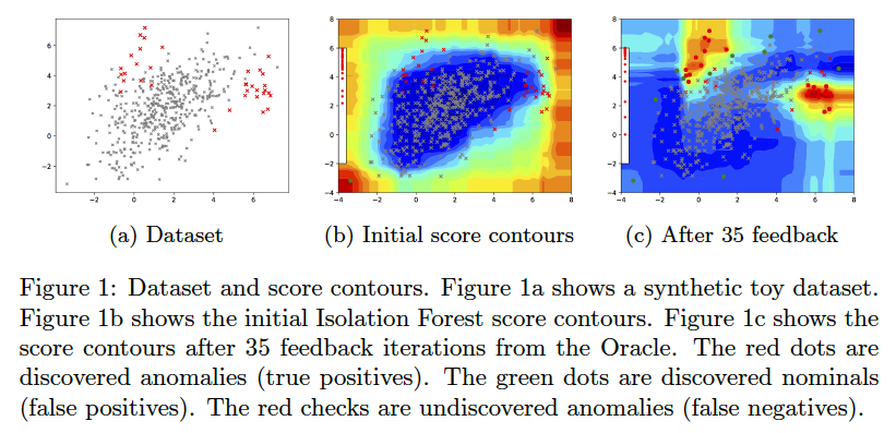
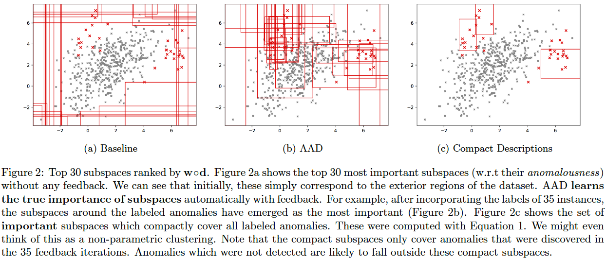
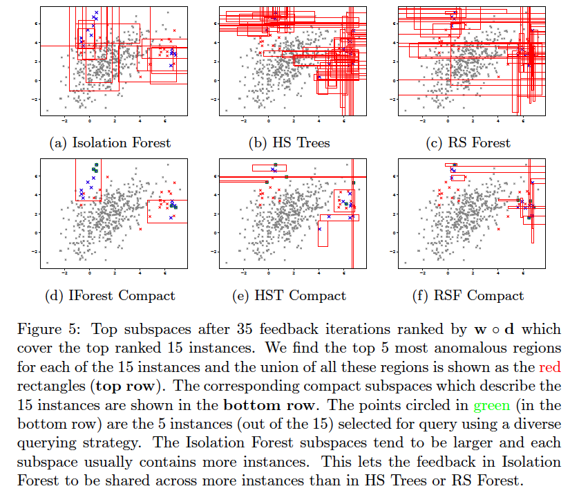
AAD, when used with a forest-based detector such as Isolation Forest, can output a compact set of subspaces that contain all labeled anomalies. The idea is explained in anomaly_description.pdf. Following illustrations show the results of this approach.

Note: The algorithm to compute compact descriptions (as illustrated here) might also be considered to be a non-parametric clustering algorithm where each 'description' is a cluster.

To generate the below, use the command:

bash ./aad.sh toy2 35 1 0.03 7 1 0 0 512 0 1 1

Applications of compact descriptions

Compact descriptions have multiple uses including:

• Discovery of diverse classes of anomalies very quickly by querying instances from different subspaces of the description
• Improved interpretability and explainability of anomalous instances

We assume that in a practical setting, the analyst(s) will be presented with instances along with their corresponding description(s). Additional information can be derived from the descriptions and shown to the analyst such as the number of instances in each description, which can help prioritize the analysis. Unfortunately, most uses of descriptions are subjective or application dependent, and therefore, hard to evaluate. However, we can evaluate the improvement in query diversity objectively as we do below.

Query diversity with compact descriptions

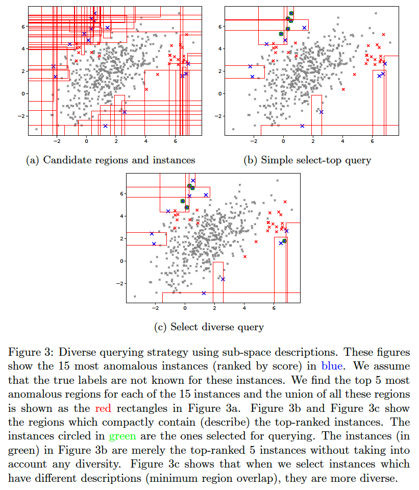
The idea for querying a diverse set of instances without significantly affecting the anomaly detection efficiency is explained in anomaly_description.pdf.

To generate the below, use the command:

bash ./aad.sh toy2 10 1 0.03 7 1 0 0 512 0 1 1

Does Query diversity with compact descriptions help?

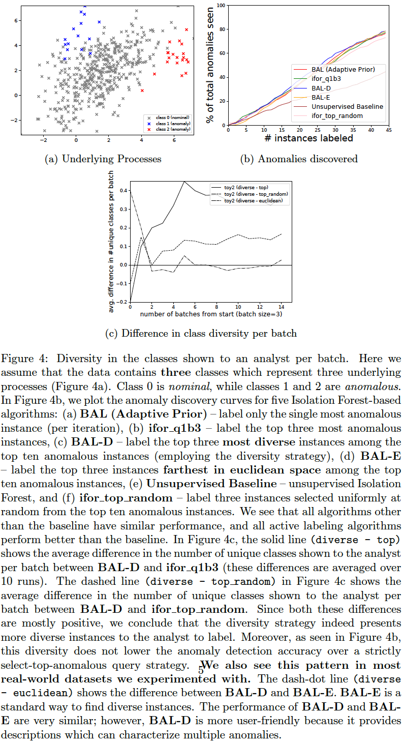
We compare the following query strategies (variables QUERY_TYPE, N_BATCH, N_EXPLORE are set in aad.sh):

• Select the single-most anomalous instance per feedback iteration: (QUERY_TYPE=1, N_BATCH=1) Select the top-most instance ordered by anomaly score. (BAL (Adaptive Prior) in the plots below.)
• Select a set of the top-most anomalous instances per feedback iteration: (QUERY_TYPE=1, N_BATCH=3) Select a batch of three top-most instances ordered by anomaly score. (ifor_q1b3 in the plots below.)
• Select a random subset of the most anomalous instances per feedback iteration: (QUERY_TYPE=2, N_BATCH=3, N_EXPLORE=10) Select a random batch of three instances among top 10 anomalous instances. (ifor_top_random in the plots below.)
• Select a subset of most anomalous instances whose descriptions are diverse within a feedback iteration: (QUERY_TYPE=8, N_BATCH=3, N_EXPLORE=10) Select three instances among top 10 anomalous instances which have most diverse descriptions (explained in previous section). (BAL-D in the plots below.)
• Select a subset of most anomalous instances which are farthest from each other within a feedback iteration: (QUERY_TYPE=9, N_BATCH=3, N_EXPLORE=10) Select three instances among the top 10 anomalous instances which have the highest average euclidean distance between them. First short-list the top 10 anomalous instances as candidates. Now, to select a batch of (three) instances, first add the most anomalous instance from these candidates to the selected list. Then iterate (two more times); in each iteration, add that instance (from the candidates) to the selected list which has the maximum average distance from the instances currently in the selected list. This is a diversity strategy common in existing literature. (BAL-E in the plots below.)

The plots below show that the description-based diversity strategy BAL-D indeed helps. While selecting the top-most anomalous instances is highly efficient for discovering anomalies, we can also improve the diversity in each query-batch through descriptions without loss in efficiency. Employing descriptions for diversity (BAL-D) also has similar query diversity on the toy2 dataset as that which maximizes the euclidean distance (BAL-E); however, the description based strategy BAL-D has the advantage of being more user-friendly because it can characterize multiple anomalies through the descriptions.

To generate the below plots, perform the following steps (remember to run the commands from the 'python' folder, and monitor progress in logs under 'python/temp' folder):

- set N_BATCH=1 in aad.sh and then run the command:

    bash ./aad.sh toy2 45 10 0.03 7 1 0 0 512 0 1 1
    
- set N_BATCH=3 in aad.sh, and run the following commands:

    bash ./aad.sh toy2 45 10 0.03 7 1 0 0 512 0 1 1
    bash ./aad.sh toy2 45 10 0.03 7 2 0 0 512 0 1 1
    bash ./aad.sh toy2 45 10 0.03 7 8 0 0 512 0 1 1
    bash ./aad.sh toy2 45 10 0.03 7 9 0 0 512 0 1 1

- Next, generate anomaly discovery curves:
    
    pythonw -m aad.plot_aad_results
    
- Finally, generate class diversity plot:

    pythonw -m aad.plot_class_diversity

Differences between Isolation Forest, HS Trees, RS Forest

This document explains why Isolation Forest is more effective in incorporating feedback at the leaf level. This is illustrated in the figure below. The plots are generated in the files query_candidate_regions_ntop5_*.pdf and query_compact_ntop5_*.pdf under temp/aad/toy2/* when the following commands are executed:

bash ./aad.sh toy2 35 1 0.03 7 1 0 0 512 0 1 1
bash ./aad.sh toy2 35 1 0.03 11 1 0 0 512 0 1 1
bash ./aad.sh toy2 35 1 0.03 12 1 0 0 512 0 1 1

Running AAD with precomputed anomaly scores

In case scores from anomaly detector ensembles are available in a CSV file, then AAD can be run with the following command.

pythonw -m aad.precomputed_aad --startcol=2 --labelindex=1 --header --randseed=42 --dataset=toy --datafile=../datasets/toy.csv --scoresfile=../datasets/toy_scores.csv --querytype=1 --detector_type=14 --constrainttype=4 --sigma2=0.5 --budget=35 --tau=0.03 --Ca=1 --Cn=1 --Cx=1 --withprior --unifprior --init=1 --runtype=simple --log_file=./temp/precomputed_aad.log --debug

Note: The detector_type is 14 for precomputed scores. The input file and scores should have the same format as in the example files (toy.csv, toy_scores.csv). Also, make sure the initialization is at uniform (--init=1) for good label efficiency (maximum reduction in false positives with minimum labeling effort). If the weights are initialized to zero or random, the results will be poor. Ensembles enable us to get a good starting point for active learning in this case.

Data Drift Detection

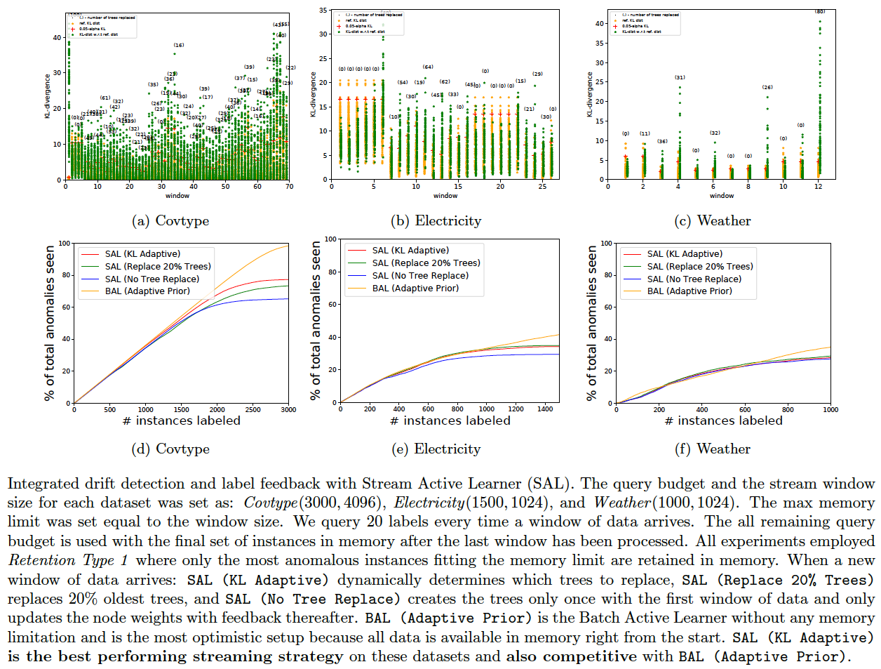
This section applies to isolation tree-based detectors (such as IForest and IForestMultiview). Such trees provide a way to compute the KL-divergence between the data distribution of one [old] batch of data with another [new] batch. Once we determine which trees have the most significant KL-divergences w.r.t expected data distributions, we can replace them with new trees constructed from new data as follows:

• First, randomly partition the current window of data into two equal parts (A and B).
• For each tree in the forest, compute average KL-divergence as follows:
  • Treat the tree as set of histogram bins
  • Compute the instance distributions with each of the data partitions A and B.
  • Compute the KL-divergence between these two distributions.
  • Do this 10 times and average.
• We now have T KL divergences where T is the number of trees.
• Compute the (1-alpha) quantile value where alpha=0.05 by default, and call this KL-q.
• Now compute the distributions for each isolation tree with the complete window of data -- call this P (P is a set of T distributions) -- and set it as the baseline.
• When a new window of data arrives replace trees as follows:
  • Compute the distribution in each isolation tree with the entire window of new data and call this Q (Q is a set of T new distributions).
  • Next, check the KL-divergences between the distributions in P and the corresponding distributions in Q. If the KL-divergence i.e., KL(p||q) of at least (2*alpha*T) trees exceed KL-q, then:
    • Replace all trees whose KL(p||q) is higher than KL-q with new trees created with the new data.
    • Recompute KL-q and the baseline distributions P with the new data and the updated model.
    • Retrain the weights certain number of times (determined by N_WEIGHT_UPDATES_AFTER_STREAM in aad.sh, 10 works well) with just the labeled data available so far (no additional feedback). This step helps tune the ensemble weights better after significant change to the model.

For more details on KL-divergence based data drift detection, check the demo code. Execute this code with the following sample command and see the plots generated (on the Weather dataset):

pythonw -m aad.test_concept_drift --debug --plot --log_file=temp/test_concept_drift.log --dataset=weather

Following shows the results of integrating drift detection along with label feedback in a streaming/limited memory setting for the three datasets (Covtype, Electricity, Weather) which we determined have significant drift. We used RETENTION_TYPE=1 in aad.sh for all datasets. The commands for generating the discovery curves for SAL (KL Adaptive) are below. These experiments will take a pretty long time to run because: (1) streaming implementation is currently not very efficient, (2) we get feedback for many iterations, and (3) we run all experiments 10 times to report an average.

bash ./aad.sh weather 1000 10 0.03 7 1 0 1 1024 1 1 1
bash ./aad.sh electricity 1500 10 0.03 7 1 0 1 1024 1 1 1
bash ./aad.sh covtype 3000 10 0.03 7 1 0 1 4096 1 1 1

The idea of partitioning the dataset to compute the KL-divergence threshold is motivated by: Tamraparni Dasu, Shankar Krishnan, Suresh Venkatasubramanian and Ke Yi, An information-theoretic approach to detecting changes in multi-dimensional data streams, Symp. on the Interface of Statistics, Computing Science, and Applications, 2006 (pdf).

Intuition behind Active Anomaly Discovery

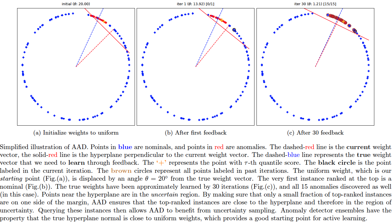
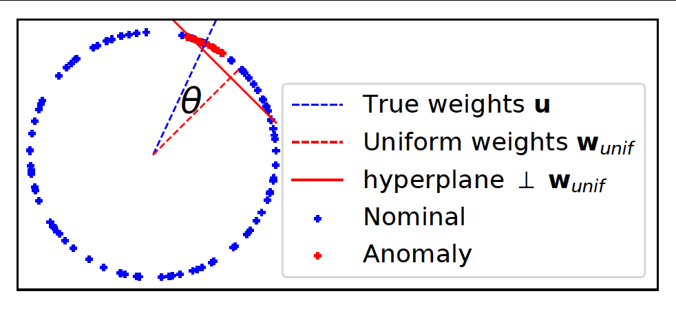
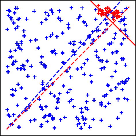
Question: Why should active learning help in anomaly detection with ensembles? Let us assume that the anomaly scores are uniformly distributed on a 2D unit sphere as in the above figure (this is a setting commonly analysed in active learning theory literature as it is easier to convey the intuition). Also assume that tau fraction of instances are anomalous. When we treat the ensemble scores as 'features', then the 'feature' vectors of anomalies will tend to be closer to the uniform unit vector than the 'feature' vectors of nominals (uniform unit vector has the same values for all 'features' and magnitude = 1). This is because anomaly detectors are designed to assign higher scores to anomalies. In other words, the dot product between the score vectors of anomalies and the uniform vector is higher than the dot product between the scores vectors of nominals and the uniform vector. (Note: the dot product of any vector with the uniform vector is equivalent to the arithmetic mean of the vector components up to a multiplicative const.) This is why combining scores by averaging works well.

Seen another way, the hyperplane perpendicular to the uniform weight vector and offset by cos(pi.tau) (in this simple 2D setting only) should be a good prior for the separating hyperplane between the anomalies and the nominals so that, ideally, anomalies lie at the extreme end -- the top right side of the hyperplane. The ideal classification rule then is: sign(w.x - cos(pi.tau)) such that +1 is anomaly, -1 is nominal. On real-world data however, the true hyperplane normal is not exactly same as the uniform vector, but should be close (else the anomaly detectors forming the ensemble are poor). AAD is basically trying to find this true hyperplane by solving a large-margin classification problem. The example percept.percept illustrates this where we have true anomaly distribution (red points in the plots) displaced by a slight angle (theta) from the uniform weights. The true hyperplane normal is represented by the blue dashed line.

With this setup, active learning can help discover the true anomaly region on the unit sphere (centered around blue dashed line) in a more efficient manner if we set the uniform vector (red dashed line) as a prior. To understand this intuitively, observe that we can design, as discussed in the previous paragraph, a hyperplane that is displaced from the origin such that a small fraction (tau) of instances are on one side and the rest are on the other side. Now, note three important observations: (1) top ranked instances are close to the hyperplane, (2) since instances close to the hyperplane have the most uncertain labels, top-ranked instances lie in the region of uncertainty (from the margin perspective), and (3) ensembles are designed so that most anomalies are top-ranked in the score-space which ensures that the uniform vector is a good prior for the hyperplane normal. Selecting top-ranked instances for labeling then results in uncertainty sampling which makes active learning efficient for learning the true hyperplane (see references below). It also makes selecting top-ranked instances for labeling efficient for discovering anomalies because: if the selected instance is truly an anomaly, it is a success; on the other hand, if the instance is a nominal, labeling it still helps to efficiently adjust the margin so that future query instances are more likely to be anomalies.

Note on the tau-based hyperplane displacement: The hyperplane displacement cos(pi.tau) is assumed only for the simple 2D scenario. In a real setting, we need to estimate the hyperplane displacement from the data, as is done by AAD. Most researchers will refer to this displacement as the bias.

Note on score normalization: By design (of ensemble members), the uniform weight vector is more closely 'hugged' by the ensemble score vectors of true anomalies than by the ensemble score vectors of nominals. However, if the score vectors are normalized to unit length (such that they all lie on a unit sphere), then this alignment is no longer guaranteed for every type of ensemble. For example, while the unit-length normalization works well for the Isolation Forest-based model with leaf nodes as the members, it does not work for the LODA-based model with the projection vectors as the members. The intuition behind AAD, as conveyed above, does not actually require the score vectors to lie on a unit sphere (not even for the Isolation Forest-based model). The general anomaly score distributions are expected to look more similar to the figure below when the anomaly scores are normalized to lie in the range [0, 1] -- as is commonly done before combining the member scores. The AAD intuition works well in this situation as well without any further unit-length normalization.

The distribution of the angles between the normalized score vectors and the uniform weight vector can be checked with aad.test_hyperplane_angles. As a recommendation: the IForest leaf-based scores may be normalized (though, not required), but LODA based scores should not be normalized to unit length.

Reference(s):

• David Cohn, Les Atlas, and Richard Ladner. Improving generalization with active learning. Machine Learning, 15(2):201–221, May 1994.
• Maria-Florina Balcan, Andrei Z. Broder, and Tong Zhang. Margin based active learning. In COLT, 2007.

Note on Spectral Clustering by label diffusion

Spectral clustering tries to first find a lower dimensional representation of the data where it is better clustered after taking into account the inherent manifold structures. Next, any standard anomaly detector can be applied on the new representation. Although the python code has the implementation, the last step requires non-metric MDS transform and the scikit-learn implementation is not as good as R. Hence, use the R code (R/manifold_learn.R) for generating the transformed features.

For details, refer to: Supervised and Semi-supervised Approaches Based on Locally-Weighted Logistic Regression by Shubhomoy Das, Travis Moore, Weng-keen Wong, Simone Stumpf, Ian Oberst, Kevin Mcintosh, Margaret Burnett, Artificial Intelligence, 2013.

Activity Modeling

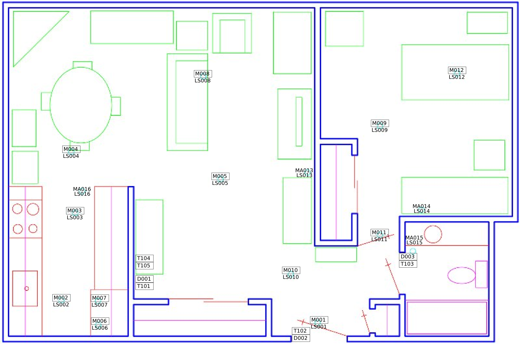
A simple application of word2vec for activity modeling can be found here. We try to infer relative sensor locations from sequence of sensor triggerings. The true floor plan and the inferred sensor locations (for sensor ids starting with 'M' and 'MA') are shown below (download the data here). This demonstrates a form of 'embedding' of the sensors in a latent space. The premise is that the non-iid data such as activity sequences may be represented in the latent space as i.i.d data on which standard anomaly detectors may be employed. We can be a bit more creative and try to apply transfer learning with this embedding.

For example, imagine that we have a house (House-1) with labeled sensors (such as 'kitchen', 'living room', etc.) and another (House-2) with partially labeled sensors. Then, if we try to reduce the 'distance' between similarly labeled sensors in the latent space (by adding another loss-component to the word2vec embeddings), it can provide more information on which of the unlabeled sensors and activities in House-2 are similar to those in House-1. Moreover, the latent space allows representation of heterogeneous entities such as sensors, activities, locations, etc. in the same space which (in theory) helps detect similarities and associations in a more straightforward manner. In practice, the amount of data and the quality of the loss function matter a lot. Moreover, simpler methods of finding similarities/associations should not be overlooked. As an example, we might try to use embedding to figure out if a particular sensor is located in the bedroom. However, it might be simpler to just use the sensor's activation time to determine this information (assuming people sleep regular hours).

Please refer to the following paper and the CASAS website for the setup: D. Cook, A. Crandall, B. Thomas, and N. Krishnan. CASAS: A smart home in a box. IEEE Computer, 46(7):62-69, 2013.