The densityratio package estimates the density ratio r(x) = p(x) / q(x) from two-samples x1 and x2 generated from two unknown distributions p(x), q(x), respectively, where x1 and x2 are d-dimensional real numbers.
The densityratio provides a densratio() class that returns an object with a function for estimating the density ratio and methods for getting the parameters of the density ratio estimation.
See the quick start for detailed usage.
The estimated density ratio function r(x) can be used in many applications such as the covariate shift adaptation, outlier detection, and change point detection. See related works.
You can install the package from GitHub
$ pip install git+https://github.com/JohnYKiyo/density_ratio_estimation.git
densityratio requires:
- Python (>= 3.6)
- Jax (>=0.1.57)
- Jaxlib (>=0.1.37)
The densityratio package includes the works (Jax, Jaxlib) that are distributed in the Apache License 2.0
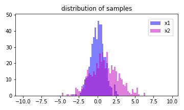
Generate two samples that follow the normal distribution of N(0,1) and N(1,2), respectively.

The code below gives the above output:
import densityratio
import numpy as np
import scipy.stats
import matplotlib.pyplot as plt
m = [0.,1]
s = [1.0,2.0]
np.random.seed(10)
x1 = np.random.normal(loc= m[0], scale = s[0], size = 500)
x2 = np.random.normal(loc= m[1], scale = s[1], size = 500)

fig = plt.figure(figsize=[5,3])
ax = fig.add_subplot(111)
ax.set_title('distribution of samples')
edges = np.arange(-10,10,0.2)
a = ax.hist(x1, bins = edges, color='b', alpha = 0.5, label='x1')
b = ax.hist(x2, bins = edges, color='m', alpha = 0.5, label='x2')
ylim = 1.1*np.max([a[0],b[0]])
ax.set_ylim(0,ylim)
ax.legend(fontsize = 10, bbox_to_anchor = (1,1), loc='upper right', borderaxespad = 1)
plt.tight_layout()
fig.savefig('pic/QS1_samples.png')Pass two samples to the densratio and it will be calculated automatically.
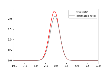
dens = densityratio.densratio(x1,x2)In this case, the true density ratio r(x) is known, so we can compare r(x) with the estimated density ratio \hat{r}(x).

The code below gives the above output:
x = np.linspace(-10,10,100)
x1_pdf = lambda x: scipy.stats.norm.pdf(x,loc=m[0],scale=s[0])
x2_pdf = lambda x: scipy.stats.norm.pdf(x,loc=m[1],scale=s[1])
r = lambda x: x1_pdf(x)/x2_pdf(x)

plt.figure()
plt.plot(x,r(x),'r',label='true ratio')
plt.plot(x,dens(x),'gray',label='estimated ratio')
plt.xlim(-10,10)
plt.legend()
plt.savefig('pic/QS1_ratio.png')
Here is this notebook
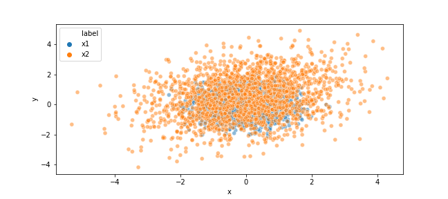
For example, Generate two samples that follow the 2-dimentional normal distribution of N(\mu_1,\Sigma_1) and N(\mu_2,\Sigma_2), respectively, and estimate the relative-densityratio [7]
r_\alpha (x) = p(x)/(\alpha p(x)+(1-\alpha)q(x)).

The code below gives the above output:
import densityratio
import numpy as np
import pandas as pd
import scipy.stats
import matplotlib.pyplot as plt
import seaborn as sns

m = [[0.,0.],[0,0.5]]
s = [np.array([[0.5,0],
                [0,0.5]]),
      np.array([[2.0,0.5],
                [0.5,2.0]])]
np.random.seed(10)
x1 = np.random.multivariate_normal(m[0], s[0], size = 2000)
x2 = np.random.multivariate_normal(m[1], s[1], size = 2000)
df = pd.DataFrame({'x':np.r_[x1[:,0],x2[:,0]],'y':np.r_[x1[:,1],x2[:,1]],'label':['x1']*len(x1)+['x2']*len(x2)})

fig = plt.figure(figsize=(9,4))
ax = fig.add_subplot(111)
sns.scatterplot(data=df, x='x', y='y', alpha=0.5,hue='label',ax=ax)
fig.savefig('pic/QS2_samples.png')If a value is set for sigma, lambda, that value is used, and if a numerical array is set, the densityratio() selects the optimum value by CV.
The alpha is a parameter that can adjust the mixing ratio, and is set in the range of [0,1.].
The kernel_number is the number of kernels in the linear model.
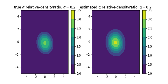
dens = densityratio.densratio(x1,x2,sigma=[0.1, 0.3, 0.5, 0.7, 1., 2., 5.], lamb=[0.01, 0.02, 0.03, 0.04, 0.05],kernel_num=200,alpha=0.2)In this case, the true density ratio r(x) with the estimated density ratio \hat{r}(x).

The code below gives the above output:
X,Y = np.meshgrid(np.linspace(-5,5,100),np.linspace(-5,5,100))
data = np.c_[X.ravel(),Y.ravel()]
x1_pdf = lambda x: scipy.stats.multivariate_normal.pdf(x,m[0],s[0])
x2_pdf = lambda x: scipy.stats.multivariate_normal.pdf(x,m[1],s[1])
Z_true = x1_pdf(data)/(0.2*x1_pdf(data)+0.8*x2_pdf(data))

fig = plt.figure(figsize=[8,4])
ax1 = fig.add_subplot(121)
ax2 = fig.add_subplot(122)
levels=np.arange(0,4,0.5)
ax1.set_title(r'true $\alpha$ relative-densityratio: $\alpha=0.2$')
ax2.set_title(r'estimated $\alpha$ relative-densityratio: $\alpha=0.2$')
a = ax1.contourf(X,Y,Z_true.reshape(100,100),levels=levels)
b = ax2.contourf(X,Y,dens(np.c_[X.ravel(),Y.ravel()]).reshape(100,100),levels=levels)
fig.colorbar(a, ax=ax1)
fig.colorbar(b, ax=ax2)
fig.savefig('pic/QS2_ratio.png')
Here is this notebook
See here
MIT License (see LICENSE).
[1] M. Suigyama et al., Direct Importance Estimation with Model Selection and Its Application to Covariate Shift Adaptation, Proc. 20th Int. Conf. Neural Inf. Process. Syst., 2007.
[2] T. Kanamori, S. Hido, and M. Sugiyama, A least-squares approach to direct importance estimation, J. Mach. Learn. Res., vol. 10, pp. 1391–1445, 2009.
[3] T. Kanamori, T. Suzuki, and M. Sugiyama, Condition number analysis of kernel-based density ratio estimation.,arXiv., (2009).
[4] S. Hido, Y. Tsuboi, H. Kashima, M. Sugiyama, and T. Kanamori, Statistical outlier detection using direct density ratio estimation, Knowl. Inf. Syst., vol. 26, no. 2, pp. 309–336, 2011.
[5] M. Sugiyama, T. Suzuki, and T. Kanamori, Density Ratio Estimation in Machine Learning. Cambridge University Press 2012.
[6] S. Liu, M. Yamada, N. Collier, and M. Sugiyama, Change-point detection in time-series data by relative density-ratio estimation, Neural Networks, 2013.
[7] M. Yamada, T. Suzuki, T. Kanamori, H. Hachiya, and M. Sugiyama, Relative density-ratio estimation for robust distribution comparison, Neural Computation. 2013.
-
uLSIF for MATLAB R C++ http://www.ms.k.u-tokyo.ac.jp/software.html
-
RuLSIF for MATLAB https://riken-yamada.github.io/RuLSIF.html
-
M. Sugiyama, M. Krauledat, and K. R. Müller, Covariate shift adaptation by importance weighted cross validation, J. Mach. Learn. Res., 2007.
-
H. Shimodaira, Improving predictive inference under covariate shift by weighting the log-likelihood function, J. Stat. Plan. Inference, 2000.
-
S. Hido, Y. Tsuboi, H. Kashima, M. Sugiyama, and T. Kanamori, Statistical outlier detection using direct density ratio estimation, Knowl. Inf. Syst., vol. 26, no. 2, pp. 309–336, 2011.
-
H. Nam and M. Sugiyama, Direct density ratio estimation with convolutional neural networks with application in outlier detection, IEICE Trans. Inf. Syst., 2015.
-
M. C. du Plessis, H. Shiino, and M. Sugiyama, Online direct density-ratio estimation applied to inlier-based outlier detection, Neural Computation. 2015.
-
Y. Kawahara and M. Sugiyama, Sequential change-point detection based on direct density-ratio estimation, Stat. Anal. Data Min., 2012.
-
S. Liu, M. Yamada, N. Collier, and M. Sugiyama, Change-point detection in time-series data by relative density-ratio estimation, Neural Networks, 2013.
-
M. Yamada, A. Kimura, F. Naya, and H. Sawada, Change-point detection with feature selection in high-dimensional time-series data, in IJCAI International Joint Conference on Artificial Intelligence, 2013.
-