Partial Derivatives Lab

Introduction

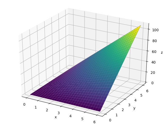
In this lesson, we'll get some more practice with partial derivatives.

Breaking down multivariable functions

In our explanation of derivatives, we discussed how taking the derivative of multivariable functions is similar to taking the derivatives of single variable functions like $f(x)$. In the first section we'll work up to taking the partial derivative of the multilinear function $ f(x,y) = 3xy $. Here's what the function looks like in a 3d graph.

Before we get there, let's first just first break this function down into it's equivalent of different slices, like we have done previously. We'll do this by taking different slices of the function, stepping through various values of $y$. So instead of considering the entire function, $f(x, y) = 3xy $ we can think about the function $f(x, y)$ evaluated at various points, where $y = 1$, $y = 3$, $y = 6$, and $y = 9$.

Write out Python functions that return the values $f(x, y)$ for $f(x, 1)$, $f(x, 3)$, $f(x, 6)$, and $f(x, 9)$ for the function $f(x, y) = 3xy $.

def three_x_y_at_one(x):
    pass

def three_x_y_at_three(x):
    pass

def three_x_y_at_six(x):
    pass

def three_x_y_at_nine(x):
    pass

three_x_y_at_one(3) # 9
three_x_y_at_three(3)# 27
three_x_y_at_six(1) # 18
three_x_y_at_six(2) # 36

Now that we have our functions written, we can write functions that provided an argument of x_values, return the associated y_values that our four functions return.

zero_to_ten = list(range(0, 11))
zero_to_four = list(range(0, 5))

def y_values_for_at_one(x_values):
    pass

def y_values_for_at_three(x_values):
    pass

def y_values_for_at_six(x_values):
    pass

def y_values_for_at_nine(x_values):
    pass

y_values_for_at_one(zero_to_four) # [0, 3, 6, 9, 12]
y_values_for_at_one(zero_to_ten) # [0, 3, 6, 9, 12, 15, 18, 21, 24, 27, 30]

y_values_for_at_three(zero_to_four) # [0, 9, 18, 27, 36]
y_values_for_at_three(zero_to_ten) # [0, 9, 18, 27, 36, 45, 54, 63, 72, 81, 90]

y_values_for_at_six(zero_to_four) # [0, 18, 36, 54, 72]
y_values_for_at_six(zero_to_ten) # [0, 18, 36, 54, 72, 90, 108, 126, 144, 162, 180]

y_values_for_at_nine(zero_to_four) # [0, 27, 54, 81, 108]
y_values_for_at_nine(zero_to_ten) #[0, 27, 54, 81, 108, 135, 162, 189, 216, 243, 270]

Now we are ready to plot the function $f(x) = x $, $f(x) = 3x $, $f(x) = 6x $ and $f(x) = 9x $

from graph import trace_values

y_at_one_trace = trace_values(zero_to_ten, y_values_for_at_one(zero_to_ten), mode = 'lines', name = 'f(x, y) at y=1') or {}

y_at_three_trace = trace_values(zero_to_ten, y_values_for_at_three(zero_to_ten),  mode = 'lines',  name = 'f(x, y) at y=3') or {}

y_at_six_trace = trace_values(zero_to_ten, y_values_for_at_six(zero_to_ten),  mode = 'lines', name = 'f(x, y) at y=6') or {}

y_at_nine_trace = trace_values(zero_to_ten, y_values_for_at_nine(zero_to_ten),  mode = 'lines', name = 'f(x, y) at y=9') or {}

import plotly
from plotly.graph_objs import Scatter, Layout
from plotly.offline import init_notebook_mode, iplot
from IPython.display import display, HTML

init_notebook_mode(connected=True)

fig_constants_lin_functions = {
    "data": [y_at_one_trace, y_at_three_trace, y_at_six_trace, y_at_nine_trace],
    "layout": Layout(title="constants with linear functions")
}
plotly.offline.iplot(fig_constants_lin_functions)

So as you can see, plotting our multivariable $f(x, y)$ at different values of $y$ above lines up conceptually to having one plot step through these values of $y$.

Evaluating the partial derivative

So in the above section, we saw how we can think of representing our multivariable functions as a function evaluated at different value of $y$.

plotly.offline.iplot(fig_constants_lin_functions)

Now let's think of how to take the derivative of our $ \frac{\partial f}{\partial x} f(x, y)$ at values of $y$. Knowing how to think about partial derivatives of multivariable functions, what is $ \frac{\partial f}{\partial x} $ at the following values of $y$.

def df_dx_when_y_equals_one():
    pass

def df_dx_when_y_equals_three():
    pass

def df_dx_when_y_equals_six():
    pass

def df_dx_when_y_equals_nine():
    pass

So notice that there is a pattern here, in taking $ \frac{\partial f}{\partial x}$ for our function $f(x, y) = 3xy$. Now write a function that calculates $ \frac{\partial f}{\partial x}$ for our function $f(x,y)$ at any provided $x$ and $y$ value.

def df_dx_3xy(x_value, y_value):
    pass

df_dx_3xy(2, 1) # 3

df_dx_3xy(2, 2) # 6

df_dx_3xy(5, 2) # 6

So as you can see, our $y$ value influences the function, and from there it's a calculation of how $f$ changes with $x$, which, in this case, is constant.

Using our partial derivative rule

Now let's consider the function $ f(x, y) = 4x^2y + 3x + y$. Now soon we will want to take the derivative of this function with respect to $x$. We know that in doing something like that, we will need to translate this function into code, and that when we do so, we will need to capture the exponent of any terms as well as.

Remember that the way we expressed a single variable function, $f(x)$ in Python was to represent the constant, and $x$ exponent for each term. For example, the function $f(x) = 3x^2 + 2x$ can be represented as the following:

three_x_squared_plus_two_x = [(3, 2), (2, 1)]

Now let's talk about representing our multivariable function $ f(x, y) =4x^2y + 3x + y$ in Python. Instead of using a tuple with two elements, we'll use a tuple with three elements and with that third element the exponent related to the $y$ variable. So our function $ f(x, y) = 4x^2y + 3x + y$ looks like the following:

four_x_squared_y_plus_three_x_plus_y = [(4, 2, 1), (3, 1, 0), (1, 0, 1)]

Let's get started by writing a function multivariable_output_at that takes in a multivariable function and returns the value $f(x, y)$ evaluated at a specific value of $x$ and $y$ for the function.

def multivariable_output_at(list_of_terms, x_value, y_value):
    pass

multivariable_output_at(four_x_squared_y_plus_three_x_plus_y, 1, 1) # 8

multivariable_output_at(four_x_squared_y_plus_three_x_plus_y, 2, 2) # 40

Let's also try this with another function $g(x, y) = 2x^3y + 3yx + x $.

two_x_cubed_y_plus_three_y_x_plus_x = [(2, 3, 1), (3, 1, 1), (1, 1, 0)]

multivariable_output_at(two_x_cubed_y_plus_three_y_x_plus_x, 1, 1) # 6

multivariable_output_at(two_x_cubed_y_plus_three_y_x_plus_x, 2, 2) # 46

So now we want to write a Python function that calculates $\frac{\partial f}{\partial x}$ of a multivariable function. Let's start by writing a function that just calculates $\frac{\partial f}{\partial x}$ of a single term.

def term_df_dx(term):
    pass

four_x_squared_y = (4, 2, 1)
term_df_dx(four_x_squared_y) # (8, 1, 1)

This solution represents $8xy$

y = (1, 0, 1)
term_df_dx(y) # (0, -1, 1)

This solution represents $0$, as the first element indicates we are multiplying the term by zero.

Now write a function that finds the derivative of all terms, $\frac{\partial f}{\partial x}$ of a function $f(x, y)$.

def df_dx(list_of_terms):
    pass

df_dx(four_x_squared_y_plus_three_x_plus_y) # [(8, 1, 1), (3, 0, 0)]

Now that we have done this for $\frac{\partial f}{\partial x}$, lets work on taking the derivative $\frac{\partial f}{\partial y}$. Once again, we can use as an example our function $ f(x, y) = 4x^2y + 3x + y$. Let's start with writing the function term_df_dy, which takes the partial derivative $\frac{\partial f}{\partial y}$ of a single term.

def term_df_dy(term):
    pass

four_x_squared_y # (4, 2, 1)

term_df_dy(four_x_squared_y) # (4, 2, 0)

This represents that $\frac{\partial f}{\partial y}4x^2y = 4x^2$

term_df_dy(y) # (1, 0, 0)

This represents that $\frac{\partial f}{\partial y}y = 1$

three_x = four_x_squared_y_plus_three_x_plus_y[1]
term_df_dy(three_x) # (0, 1, -1)

This represents that $\frac{\partial f}{\partial y}3x = 0$

Now let's write a function df_dy that takes multiple terms and returns an list of tuples that represent the derivative of our multivariable function. So here is our function: $ f(x, y) = 4x^2y + 3x + y$.

four_x_squared_y_plus_three_x_plus_y

def df_dy(list_of_terms):
    pass

df_dy(four_x_squared_y_plus_three_x_plus_y) # [(4, 2, 0), (1, 0, 0)]

two_x_cubed_y_plus_three_y_x_plus_x = [(2, 3, 1), (3, 1, 1), (1, 1, 0)]
df_dy(two_x_cubed_y_plus_three_y_x_plus_x) # [(2, 3, 0), (3, 1, 0)]

Great job! Hopefully, now you understand a little more about multivariable functions and derivatives!

worldyne/partial-derivatives-lab-data-science-intro-000

Partial Derivatives Lab

Introduction

Breaking down multivariable functions

Evaluating the partial derivative

Using our partial derivative rule