This is the GitHub repository for the Sentinel-1 and Sentinel-2 dataset Tropical Tree Cover, which is viewable on Google Earth Engine here. The asset is public as of May 2023 on Google Earth Engine here. The dataset is published in Remote Sensing of Environment. The models are released as nonfrozen Tensorflow 1.15.4 graphs and frozen Tensorflow 1.15 & Tensorflow 2.X (tested with 2.13.x) graphs in the models-release/ folder.
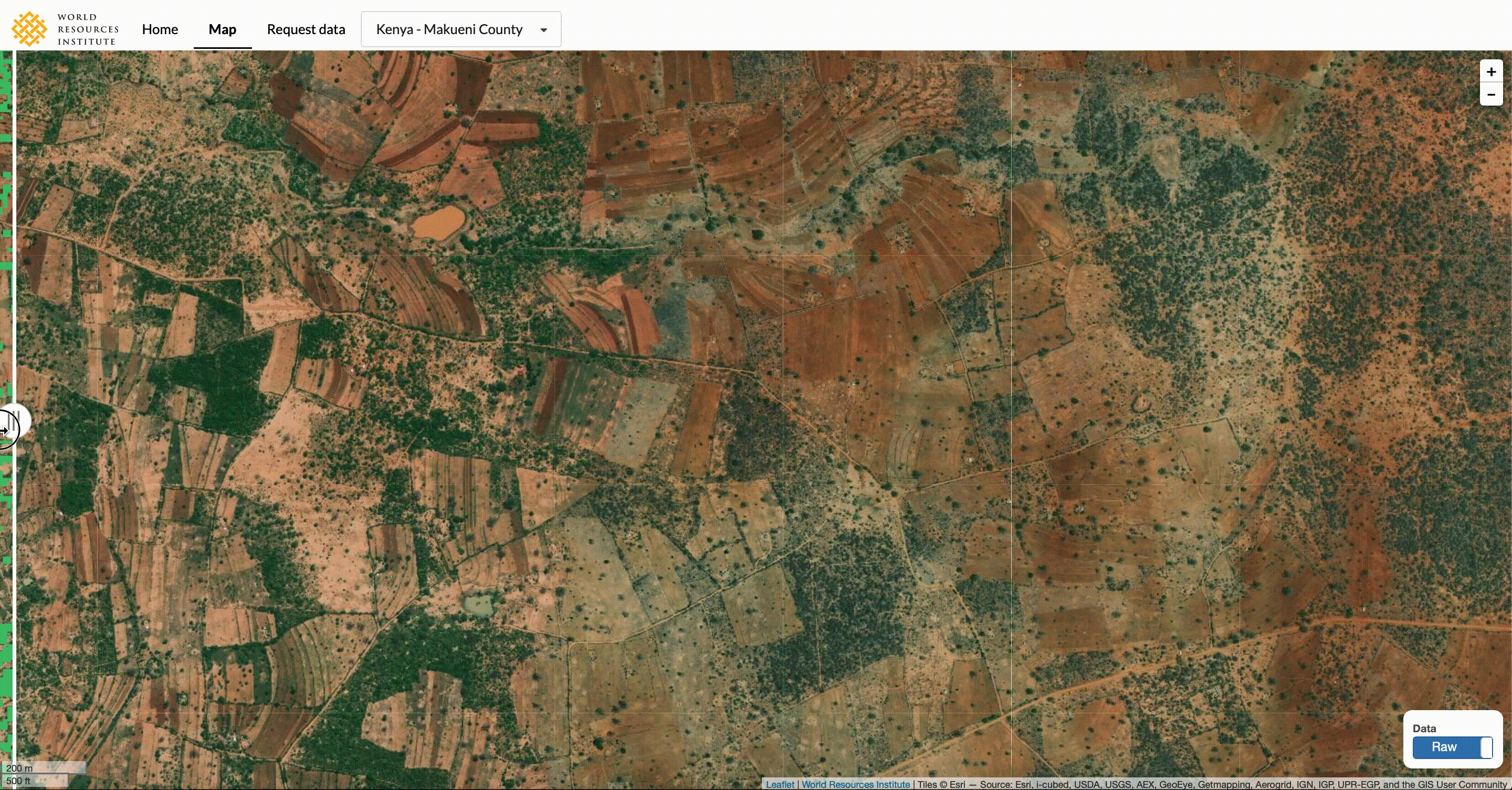
This project maps tree extent at the ten-meter scale using open source artificial intelligence and satellite imagery. The data enables accurate reporting of tree cover in urban areas, tree cover on agricultural lands, and tree cover in open canopy and dry forest ecosystems.
This repository contains the source code for the project. A full description of the methodology can be found in the publication. The data product specifications can be accessed on the wiki page.
- Background
- Data Extent
- Methodology
- Validation and Analysis | Jupyter Notebook
- Definitions
- Limitations
We have released the model files to allow users to either directly run inference or to finetune the model with their own training data. Because the models were originally developed in the mostly deprecated Tensorflow 1 API, there are some peculiarities that need to be understood for use.
We have released nonfrozen files for Tensorflow 1.15.4 here. These files can be used to finetune/continue training the model with the Tensorflow 1 saver API using saver.restore(sess, tf.train.latest_checkpoint(path)). This file requires the input to be (5, 28, 28, 17) shape and normalized using the mins and maxes found here.
We have released frozen files for Tensorflow2.X here. The numbers at the end of the file names correspond to the size of the output image, which is always 14 less than the size of the input (e.g. 172 x 172 output for 186 x 186 input). The frozen weights can be loaded into TF1/2 API using the approach here and the input images should be normalized following the code here.
Unfortunately, after a lot of testing, some of the critical model modules (modified ConvGRU with attention, partial convolution, and modified normalization within the ConvGRU cells, DropBlock) do not properly train in Tensorflow 2.X, even after our best attempts at porting them to the TF2.X API. This seems to be due to how the gradient is calculated in TF2 vs TF1, and does not affect frozen graphs for inference. However, finetuning in Tensorflow 2 will not work.
We have also tested porting the model to Pytorch, see here but similarily, Zoneout, which is a critical regularizer for the ConvGRU, does not exist in Pytorch. The resulting maps generated in Pytorch are not good despite verifying the same model structure, optimizer, training data, etc, so as of May 2024 there is no working Pytorch version.
As of July 2024, the Tensorflow 1.X training files are released in the src/train file. There is an args dictionary in train-model.py that can be adjusted to retrain the model for your own needs.
Brandt, J., Ertel, J., Spore, J., & Stolle, F. (2023). Wall-to-wall mapping of tree extent in the tropics with Sentinel-1 and Sentinel-2. Remote Sensing of Environment, 292, 113574. doi:10.1016/j.rse.2023.113574
Brandt, J. & Stolle, F. (2021) A global method to identify trees outside of closed-canopy forests with medium-resolution satellite imagery. International Journal of Remote Sensing, 42:5, 1713-1737, DOI: 10.1080/01431161.2020.1841324
An overview Jupyter notebook walking through the creation of the data can be found here
An example Google Earth Engine script to export Geotiffs of the extent data by country can be found here and an example script to export Geotiffs by AOI can be found here
Utilizing this repository to generate your own data requires:
- Sentinel-Hub API key, see Sentinel-hub
- Amazon Web Services API key (optional) with s3 read/write privileges
The API keys should be stored as config.yaml in the base directory with the structure:
key: "YOUR-SENTINEL-HUB-API-KEY"
awskey: "YOUR-AWS-API-KEY"
awssecret: "YOUR-AWS-API-SECRET"
The code can be utilized without AWS by setting --ul_flag False in download_and_predict_job.py. By default, the pipeline will output satellite imagery and predictions in 6 x 6 km tiles to the --s3_bucket bucket. NOTE: The specific layer configurations for Sentinel-Hub have not yet been released but are available on request.
git clone https://github.com/wri/sentinel-tree-cover
cd sentinel-tree-cover/
touch config.yaml
vim config.yaml # insert your API keys here
docker build -t sentinel_tree_cover .
docker run -it --entrypoint /bin/bash sentinel_tree_cover:latest
cd src
python3 download_and_predict_job.py --country "country" --year year
- Clone repository
- Install dependencies
pip3 install -r requirements.txt - Install GDAL (different process for different operating systems, see https://gdal.org)
- Download model
python3 src/models/download_model.py - Start Jupyter notebook and navigate to
notebooks/folder
The notebooks/ folder contains ordered notebooks for downloading training and testing data and training the model, as follows:
- 1a-download-sentinel-2: downloads monthly mosaic 10 and 20 meter bands for training / testing plots
- 1b-download-sentinel-1: downloads monthly VV-VH db sigma Sentinel-1 imagery for training / testing plots
- 2-data-preprocessing: Combines satellite imagery for training / testing plots with labelled data from Collect Earth Online
- 3-feature-selection: Feature selection for remote sensing indices utilizing random forests
- 4-model: Trains and deploys tree cover model
The src/ folder contains the source code for the project, as well as the primary entrypoint for the Docker container, download_and_predict_job_fast.py
download_and_predict_job_fast.py can be used as follows, with additional optional arguments listed in the file: python3 download_and_predict_job_fast.py --country $COUNTRY --year $YEAR
This model uses a U-Net architecture with the following modifications:
- Convolutional GRU encoder with group normalization to develop temporal features of monthly cloud-free mosaics
- Concurrent spatial and channel squeeze excitation in both the encoder and decoder (https://arxiv.org/abs/1803.02579)
- DropBlock and Zoneout for generalization in both the encoder and decoder
- Group normalization and Swish activation in both the encoder and decoder
- AdaBound optimizer with Stochastic Weight Averaging and Sharpness Aware Minimization
- Binary cross entropy and boundary loss
- Smoothed image predictions across moving windows with Gaussian filters
- A much larger input (28x28) than output (14x14) at training time, with 182x182 and 168x168 input and output size in production, respectively

This project uses Sentinel 1 and Sentinel 2 imagery. Monthly composites of Sentinel 1 VV-VH imagery are fused with the nearest Sentinel 2 10- and 20-meter bands. These images are preprocessed by:
- Super-resolving 20m bands to 10m with DSen2
- Calculating cloud cover and cloud shadow masks
- Removing steps with >30% cloud cover, and linearly interpolating to remove clouds and shadows from <30% cloud cover images
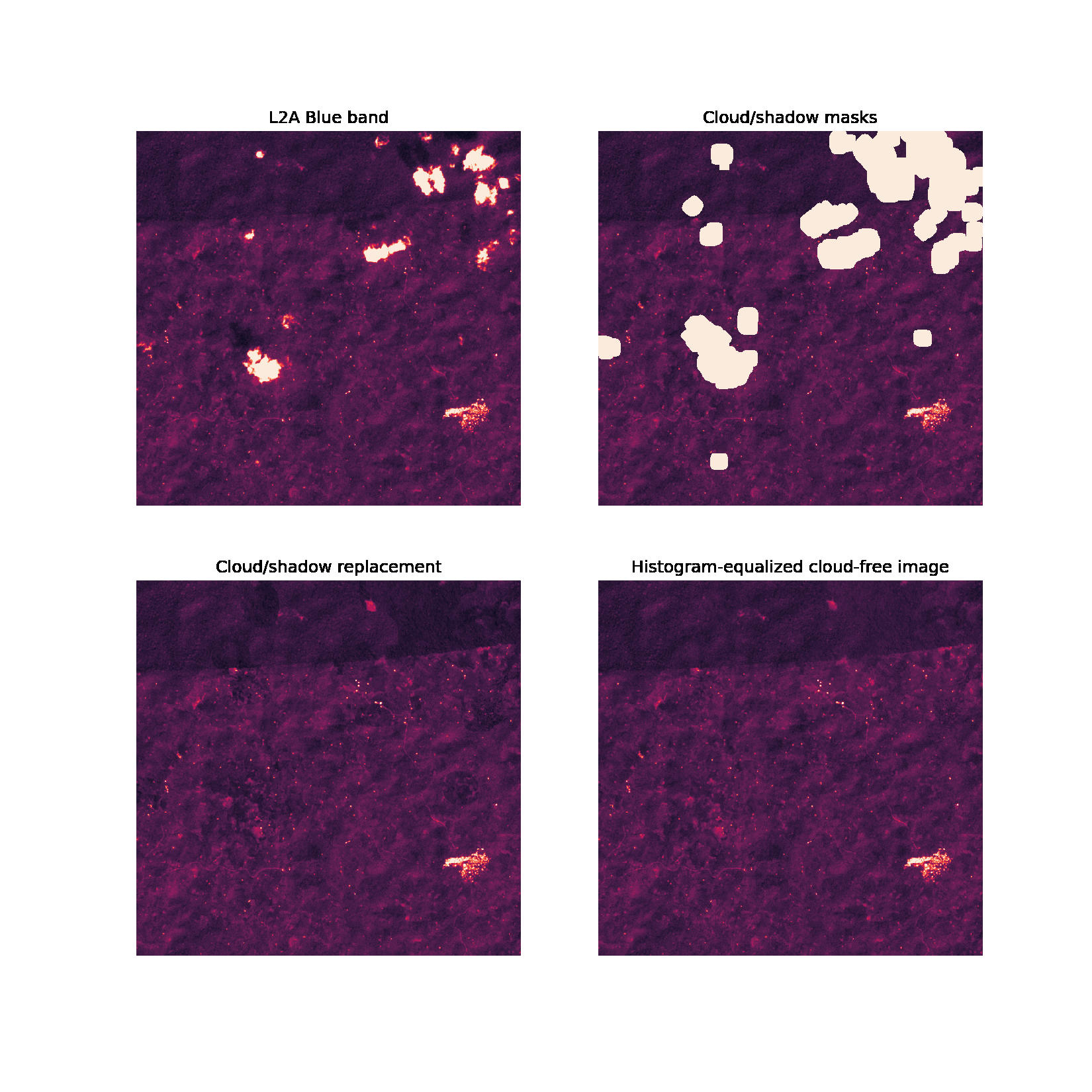
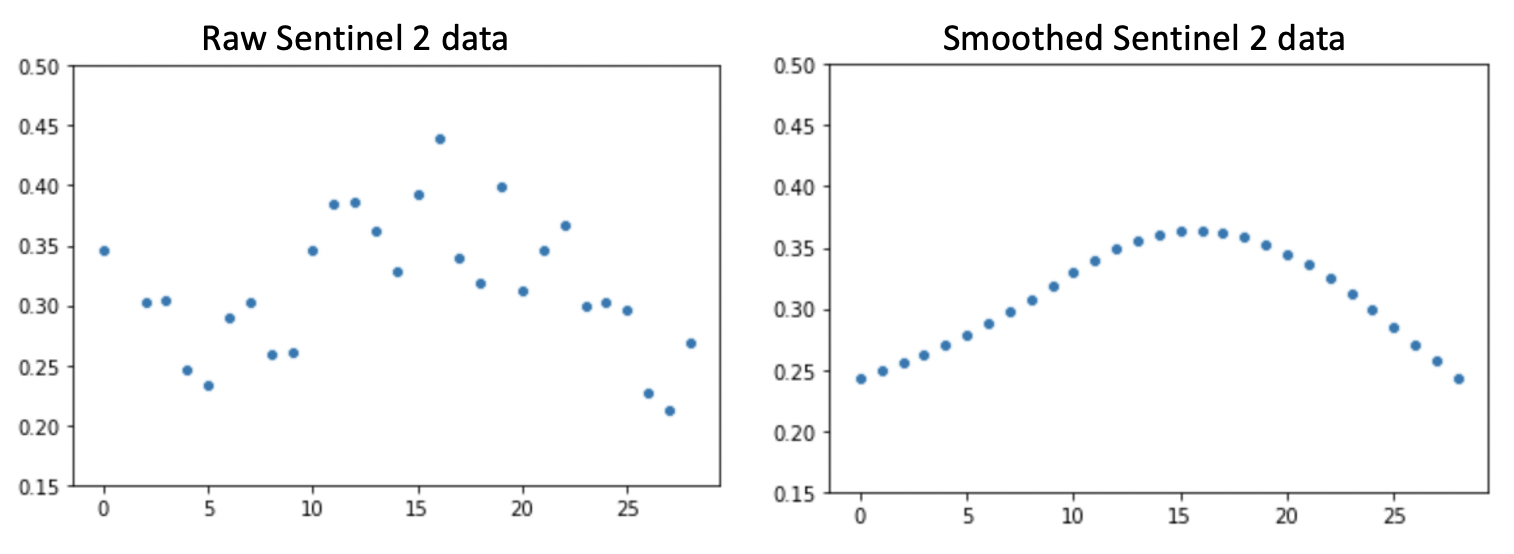
- Applying Whittaker smoothing (lambda = 100) to each time series for each pixel for each band to reduce noise
- Calculating vegetation indices, including EVI, BI, and MSAVI2


The cloud / shadow removal and temporal mosaicing algorithm is summarized below:
- Select all images with <30% cloud cover
- Select up to two images per month with <30% cloud cover, closest to beginning and middle of month
- Select least cloudy image if max CC > 15%, otherwise select the image closest to the middle of the month
- Linearly interpolate clouds and cloud shadows with a rolling median
- Smooth time series data with a rolling median
- Linearly interpolate image stack to a 15 day timestep
- Smooth time stack with Whittaker smoother
The following configurations are necessary to utilize data exported from Sentinel Hub.
- L2A20_ORBIT: Bands 5, 6, 7, 8a at 20m resolution L2A, orbit mosaic
- L2A40_ORBIT: Bands 11, 12 at 40m resolution L2A, orbit mosaic (processed at 40m instead of 20m to save storage)
- L2A10_ORBIT: 10-meter bands L2A, orbit mosaic
- CLOUD_SCL_PREVIEW: Very low resolution cloud masks used to select image dates
- DATA_QUALITY: Identifies images to acquire based on image angles, aerosol optical thickness
- CIRRUS_CLOUDS: Identifies images to acquire based on cirrus masks
L2A20_ORBIT
//VERSION=3 (auto-converted from 1) + dataMask to control background color + scaling to UINT16 range

function setup() {
  return {
    input: [{
      bands: [
        "B05",
        "B06",
        "B07",
        "B8A",
        "dataMask",
             ]
    }],
    mosaicking: Mosaicking.ORBIT,
    output: {
      id: "default",
      bands: 4,
      sampleType:"UINT16",

    }
  }
}


function evaluatePixel(samples, scenes, inputMetadata, customData, outputMetadata) {
  //Average value of band B02 based on the requested scenes
  var b05 = 1
  var b06 = 1
  var b07 = 1
  var b8a = 1
  for (i = 0; i < samples.length; i++) {
    var sample = samples[i]
    if (sample.dataMask == 1){
        if (sample.B05 < b05) {
          b05 = sample.B05
          b06 = sample.B06
          b07 = sample.B07
          b8a = sample.B8A
        }
    }
  }
  return [b05 * 65535, b06 * 65535, b07 * 65535, b8a * 65535]
}

function updateOutputMetadata(scenes, inputMetadata, outputMetadata) {
  outputMetadata.userData = {
    "inputMetadata": inputMetadata
  }
  outputMetadata.userData["orbits"] = scenes.orbits
}
L2A10_ORBIT
//VERSION=3
function setup() {
  return {
    input: ["B02", "B03", "B04", "B08", "dataMask"],
    mosaicking: Mosaicking.ORBIT,
    output: {
      id: "default",
      sampleType:"UINT16",
      bands: 4
    }
  }
}

function evaluatePixel(samples, scenes, inputMetadata, customData, outputMetadata) {
  //Average value of band B02 based on the requested scenes
  var sumOfValidSamplesB02 = 0
  var numberOfValidSamples = 0
  var b02 = 1
  var b03 = 1
  var b04 = 1
  var b08 = 1
  for (i = 0; i < samples.length; i++) {
    var sample = samples[i]
    if (sample.dataMask == 1){
        if (sample.B02 < b02) {
          b02 = sample.B02
          b03 = sample.B03
          b04 = sample.B04
          b08 = sample.B08
        }
    }
  }
  return [b02 * 65535, b03 * 65535, b04 * 65535, b08 * 65535]
}

function updateOutputMetadata(scenes, inputMetadata, outputMetadata) {
  outputMetadata.userData = {
    "inputMetadata": inputMetadata
  }
  outputMetadata.userData["orbits"] = scenes.orbits
}
L2A40_ORBIT
//VERSION=3 (auto-converted from 1) + dataMask to control background color + scaling to UINT16 range

function setup() {
  return {
    input: [{
      bands: [
        "B11",
        "B12",
        "dataMask",
             ]
    }],
    mosaicking: Mosaicking.ORBIT,
    output: {
      id: "default",
      bands: 3,
      sampleType:"UINT16",

    }
  }
}


function evaluatePixel(samples, scenes, inputMetadata, customData, outputMetadata) {
  //Average value of band B02 based on the requested scenes
  var b11 = 1
  var b12 = 1
  for (i = 0; i < samples.length; i++) {
    var sample = samples[i]
    if (sample.dataMask == 1){
        if (sample.B11 < b11) {
          b11 = sample.B11
          b12 = sample.B12
        }
    }
  }
  return [b11 * 65535, b12 * 65535]
}

function updateOutputMetadata(scenes, inputMetadata, outputMetadata) {
  outputMetadata.userData = {
    "inputMetadata": inputMetadata
  }
  outputMetadata.userData["orbits"] = scenes.orbits
}
CLOUD_SCL_PREVIEW
//VERSION=3 (auto-converted from 1) + dataMask to control background color + scaling to UINT16 range
function evaluatePixel(samples) {
    var factor = 255
    if (samples.dataMask == 0) {
      return [255]
    } else if ((samples.CLP / 255) > 0.7) {
      return [100]
    } else {
    return [0];
    }
}
function setup() {
  return {
    input: [{
      bands: [
        "dataMask",
        "CLP",
             ]
    }],
    output: {
      bands: 1,
      sampleType:"UINT8",
      mosaicking: "ORBIT"
    }
  }
}
DATA_QUALITY
//VERSION=3 (auto-converted from 1) + dataMask to control background color + scaling to UINT16 range

function evaluatePixel(samples) {
    var factor = 255
    if (samples.dataMask == 0) {
      return [255]
    } else if (samples.AOT > 0.6) {
      return [255]
    } else if (samples.sunZenithAngles < 13) {
      return [255]
    } else if (samples.viewZenithMean > 12) {
      return [255]
    } else {
    return [0];
    }
}
function setup() {
  return {
    input: [{
      bands: [
        "dataMask",
        "viewZenithMean",
        "sunZenithAngles",
        "AOT",
             ]
    }],
    output: {
      bands: 1,
      sampleType:"UINT8",
      mosaicking: "ORBIT"
    }
  }
}
CIRRUS_CLOUDS
//VERSION=3 (auto-converted from 1) + dataMask to control background color + scaling to UINT16 range
function setup() {
  return {
    input: ["B02", "CLP", "dataMask"],
    mosaicking: Mosaicking.ORBIT,
    output: {
      id: "default",
      sampleType:"UINT16",
      bands: 1
    }
  }
}

function evaluatePixel(samples, scenes, inputMetadata, customData, outputMetadata) {
  //Average value of band B02 based on the requested scenes
  var sumOfValidSamplesB02 = 0
  var numberOfValidSamples = 0
  var b02 = 1
  var scl = 0.
  for (i = 0; i < samples.length; i++) {
    var sample = samples[i]
    if (sample.dataMask == 1){
        if (sample.B02 < b02) {
          b02 = sample.B02
          if (sample.CLP > (255 * 0.67)) {
          	scl = 2
          }
        }
    }
  }
  return [scl]
}

function updateOutputMetadata(scenes, inputMetadata, outputMetadata) {
  outputMetadata.userData = {
    "inputMetadata": inputMetadata
  }
  outputMetadata.userData["orbits"] = scenes.orbits
}
The code is released under the GNU General Public License v3.0.
├── LICENSE
├── Makefile           <- Makefile with commands like `make data` or `make train`
├── README.md          <- The top-level README for developers using this project.
├── docs               <- A default Sphinx project; see sphinx-doc.org for details
│
├── models             <- Trained and serialized models, model predictions, or model summaries
│
├── notebooks          <- Jupyter notebooks
│   └── baseline
│   └── replicate-paper
│   └── visualization
│
├── references         <- Data dictionaries, manuals, and all other explanatory materials.
│
├── requirements.txt   <- The requirements file for reproducing the analysis environment, e.g.
│                         generated with `pip freeze > requirements.txt`
│
├── setup.py           <- makes project pip installable (pip install -e .) so src can be imported
├── src                <- Source code for use in this project.
│   ├── __init__.py    <- Makes src a Python module
│   │
│   ├── data           <- Scripts to download or generate data
│   │   └── make_dataset.py
│   │
│   ├── features       <- Scripts to turn raw data into features for modeling
│   │   └── build_features.py
│   │
│   ├── models         <- Scripts to train models and then use trained models to make
│   │   │                 predictions
│   │   ├── predict_model.py
│   │   └── train_model.py
│   │
│   └── visualization  <- Scripts to create exploratory and results oriented visualizations
│       └── visualize.py
│
└── tox.ini            <- tox file with settings for running tox; see tox.testrun.org