hbcm package

Community detection is a clustering method based on objects’ pairwise relationships such that objects classified in the same group are more densely connected than objects from different groups and correlations within the same cluster are homogeneous. Most of the model-based community detection methods such as the stochastic block model and its variants are designed for networks with binary (yes/no) connectivity values, which ignores the practical scenarios where the pairwise relationships are continuous, reflecting different degrees of connectivity. The heterogeneous block covariance model (HBCM) proposes a novel clustering structure applicable on signed and continuous connections, such as the covariances or correlations between objects. Furthermore, it takes into account the heterogeneous property of each object within a community. A novel variational EM algorithm is employed to estimate the optimal group membership. HBCM has provable consistent estimation of clustering memberships and its practical performance is demonstrated by numerical simulations. The HBCM is illustrated on yeast gene expression data and gene groups with correlated expression levels responding to the same transcription factors are detected.

Installation

You can install the development version from GitHub with:

# install.packages("devtools")
devtools::install_github("xiangli2pro/hbcm")

# load package
library('hbcm')

Examples

1. Simulation data

Create a matrix data x of dimension NxP=1000x500, with columns belonging to five (K=5) non-overlapping groups (groups labeled as 1 to 5). x values are determined by three things: parameter vector alpha of size NxK (follows multivariate normal distribution), heterogeneous parameters vector hlambda and hsigma of sizes Px1 respectively.

# check function arguments and return values documentation
?hbcm::data_gen

# x dimension
n <- 500
p <- 500

# cluster number
centers <- 5
# cluster labels follow a multinulli distribution with probability ppi
ppi <- rep(1/centers, centers)
# simulate a vector of labels from the multinulli distribution
labels <- sample(c(1:centers), size = p, replace = TRUE, prob = ppi) 

# specify the (mu, omega) of the MVN distribution of alpha
mu <- rep(0, centers)

off_diag <- 0.5
omega <- diag(rep(1, centers))
for (i in 1:centers) {
  for (j in 1:centers) {
    if (i!=j){
      omega[i,j] = off_diag
    } 
  }
}

# set up the generating function of hlambda and hsigma
hparam_func <- list(
  lambda_func = function(p) stats::rnorm(p, 0, 1),
  sigma_func = function(p) stats::rchisq(p, 2) + 1
)

# set up the number of simulation data
size <- 1

# generate data
data_list <- hbcm::data_gen(n, p, centers, mu, omega, labels, size, hparam_func)
x <- data_list$x_list[[1]]

2. Cluster the columns into `K` groups

Use heterogeneous block covariance model (HBCM) to cluster the columns of data x. Need to provide a starting label guess and the number of clusters.

# check function arguments and return values documentation
?hbcm::heterogbcm()

# use spectral clustering to make a label guess
start_labels <- kernlab::specc(abs(cor(x)), centers = centers)@.Data


# use hbcm to perform clustering
hbcm_res <- hbcm::heterogbcm(x, centers = centers, 
                tol = 1e-3, iter = 100, iter_init = 3, 
                labels = start_labels, 
                verbose = FALSE)

3. Evaluate the clustering performance

Use metric Rand-Index and adjusted Rand-Index to compare the estimated label assignment with the true label assignment. The higher the value, the better the performance.

# check function arguments and return values documentation
?hbcm::matchLabel()

# evaluate clustering performance
library('dplyr')
specc_eval <- hbcm::matchLabel(labels, start_labels) %>% 
  unlist() %>% round(3)
hbcm_eval <- hbcm::matchLabel(labels, hbcm_res$cluster) %>% 
  unlist() %>% round(3)

# result shows that hbcm model is better than spectral-clustering model in terms of rand index.
print(specc_eval)
#>    Rand adjRand 
#>   0.614   0.059
print(hbcm_eval)
#>    Rand adjRand 
#>   0.790   0.401

Miscellaneous

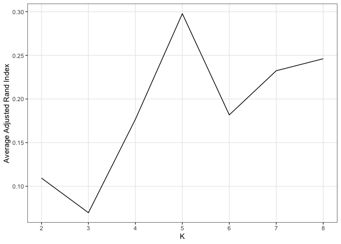
1. Use cross-Validation to select `K` when it’s unknown

In practice the number of clusters is often unknown, in which case we recommend to use the cross-validation with adjusted rand index as standard to select the K. The optimalK is achieved at the highest adjusted rand index.

lapply(c("parallel", "foreach", "doParallel", "tidyverse"), require, char=TRUE)
#> [[1]]
#> [1] TRUE
#> 
#> [[2]]
#> [1] TRUE
#> 
#> [[3]]
#> [1] TRUE
#> 
#> [[4]]
#> [1] TRUE

registerDoParallel(detectCores())
kVec <- c(2:8)
cv_res <- foreach(K = kVec,.errorhandling = 'pass',
               .packages = c("MASS","Matrix","matrixcalc","kernlab", "RSpectra")) %dopar%
  hbcm::crossValid_func_adjR(x, centers = K, pt = 10)

# summary & plot
data.frame(kVec, unlist(cv_res)) %>% 
  `colnames<-`(c("K", "adjR")) %>%
  ggplot() +
  geom_line(aes(x = K, y = adjR))+
  xlab("K")+
  ylab("Average Adjusted Rand Index")+
  theme_bw() +
  theme(panel.grid.minor = element_blank()) +
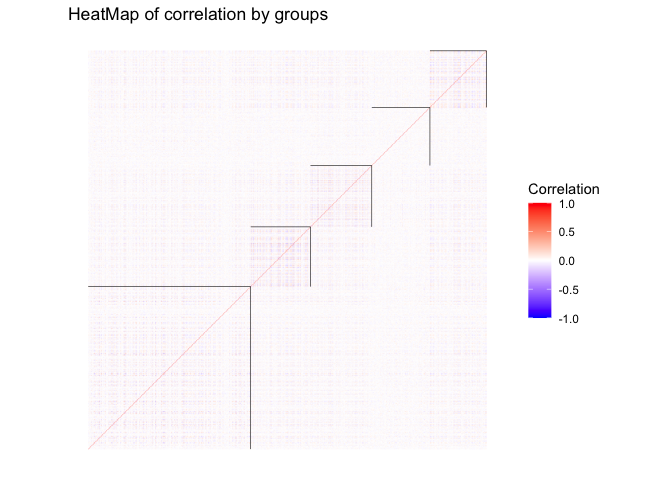
  scale_x_continuous(breaks =kVec)

2. Use heatmap to display the group structure

hbcm::colMat_heatMap(
  affMatrix = cor(x), centers, labels = hbcm_res$cluster,
  margin = 0.5, midpoint = 0, limit = c(-1,1), size = 0.2,
  legendName = "Correlation", title = "HeatMap of correlation by groups")

xiangli2pro/hbcm