Using The Super-Resolution Convolutional Neural Network for Image Restoration

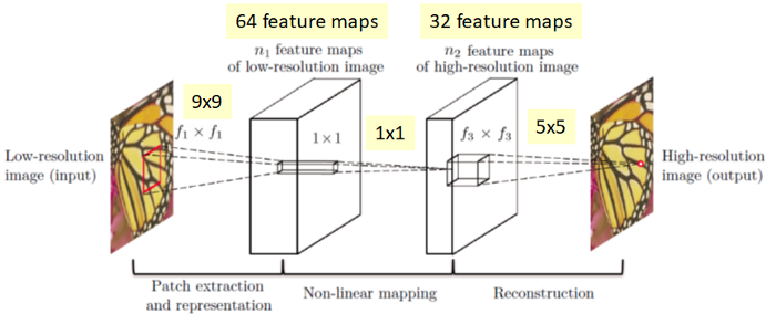
Using The Super-Resolution Convolutional Neural Network for Image Restoration
The SRCNN Network
1. Importing Packages
- Import the necessary packages
2. Image Quality Metrics
3. Preparing Images
3. Testing Low-Resolution Images
4. Building the SRCNN Model
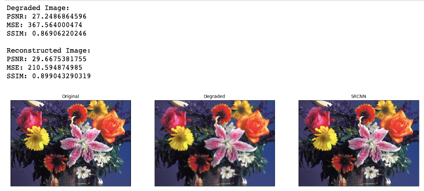
5. Deploying the SRCNN

Welcome to this comprehensive tutorial on single-image super-resolution (SR). In this tutorial, we will delve into the fascinating world of image enhancement and the techniques that allow us to recover high-resolution details from low-resolution inputs, a concept often dramatized in modern crime shows as "enhancing" images.

What is Single-Image Super-Resolution?

Single-Image Super-Resolution, often abbreviated as SR, is a field in image processing and computer vision that focuses on the task of enhancing the spatial resolution of an image. It involves taking a low-resolution image and generating a high-resolution version of it. This process is invaluable in various applications, such as improving the quality of images captured by surveillance cameras, enhancing medical images, or upscaling old, low-quality photographs.

The Super-Resolution Convolutional Neural Network (SRCNN)

To achieve the remarkable goal of SR, we will employ a powerful tool known as the Super-Resolution Convolutional Neural Network, or SRCNN for short. The SRCNN is a deep convolutional neural network architecture that has significantly advanced the field of SR. It was introduced in the groundbreaking paper titled "Image Super-Resolution Using Deep Convolutional Networks" by Chao Dong, et al. in 2014. You can explore the full details of this paper on https://arxiv.org/abs/1501.00092..

Key Features of SRCNN:

End-to-End Learning: SRCNN is designed to learn the complex mapping from low-resolution to high-resolution images directly from data. It excels at capturing intricate details during the super-resolution process. Image Quality Metrics: To quantify the performance of the SRCNN and the quality of the enhanced images, we will employ three fundamental image quality metrics: Peak Signal-to-Noise Ratio (PSNR), Mean Squared Error (MSE), and the Structural Similarity (SSIM) index. These metrics provide quantitative insights into the effectiveness of SR techniques. Why Single-Image Super-Resolution Matters

In essence, the significance of SR lies in its ability to enhance the quality and detail of images, even when the original data is low-resolution. This has transformative implications for a wide range of applications, enabling us to obtain sharper, more detailed images from sources that were previously limited by their resolution.

For instance, imagine the capability to extract crucial details from a grainy security camera feed or to restore the clarity of historical photographs. These are just a few examples of the remarkable real-world applications of SR techniques.

In this tutorial, we will walk you through the entire process of implementing and deploying the SRCNN model using Keras. You will gain hands-on experience in using SR to enhance images and learn how to evaluate the results using objective quality metrics.

Now, let's embark on this exciting journey into the world of single-image super-resolution, where we will uncover the techniques, code, and concepts that make it all possible.

Furthermore, we will be using OpenCV, the Open Source Computer Vision Library. OpenCV was originally developed by Intel and is used for many real-time computer vision applications. In this particular project, we will be using it to pre and post process our images. As you will see later, we will frequently be converting our images back and forth between the RGB, BGR, and YCrCb color spaces. This is necessary because the SRCNN network was trained on the luminance (Y) channel in the YCrCb color space.

During this project, you will learn how to:

use the PSNR, MSE, and SSIM image quality metrics,
process images using OpenCV,
convert between the RGB, BGR, and YCrCb color spaces,
build deep neural networks in Keras,
deploy and evaluate the SRCNN network

The SRCNN Network

1. Importing Packages

Let’s dive right in! This section imports the necessary libraries and packages for the project and prints their version numbers to ensure compatibility. It includes common libraries like Keras, OpenCV, NumPy, Matplotlib, and scikit-image. This is an important step to make sure we are all on the same page; furthermore, it will help others reproduce the results we obtain.

# check package versions

# Check package versions
import sys
import keras
import cv2
import numpy
import matplotlib
import skimage

print('Python:', sys.version)
print('Keras:', keras.__version__)
print('OpenCV:', cv2.__version__)
print('NumPy:', numpy.__version__)
print('Matplotlib:', matplotlib.__version__)
print('Scikit-Image:', skimage.__version__)

Import the necessary packages

import sys
import keras
import cv2
import numpy as np
import math
import os
from keras.models import Sequential
from keras.layers import Conv2D
from keras.optimizers import Adam
from skimage.measure import compare_ssim as ssim
import matplotlib.pyplot as plt

# python magic function, displays pyplot figures in the notebook
%matplotlib inline

2. Image Quality Metrics

To start, let's define a couple of functions that we can use to calculate the PSNR, MSE, and SSIM. The structural similarity (SSIM) index was imported directly from the scikit-image library; however, we will have to define our own functions for the PSNR and MSE. Furthermore, we will wrap all three of these metrics into a single function that we can call later.

2.1. PSNR (Peak Signal-to-Noise Ratio)

PSNR measures the quality of an image by comparing it to a reference image. It's a widely used metric in image processing and computer vision.

Example:

# define a function for peak signal-to-noise ratio (PSNR)

# Image Quality Metrics
def psnr(target, ref):
    # assume RGB image
    target_data = target.astype(float)
    ref_data = ref.astype(float)

    diff = ref_data - target_data
    diff = diff.flatten('C')

    rmse = math.sqrt(np.mean(diff ** 2.))

    return 20 * math.log10(255. / rmse)

2.2. MSE (Mean Squared Error)

MSE calculates the average squared difference between the pixels of two images. It provides a measure of the average squared intensity difference between the target and reference images.

# define function for mean squared error (MSE)

def mse(target, ref):
    # the MSE between the two images is the sum of the squared difference between the two images
    err = np.sum((target.astype('float') - ref.astype('float')) ** 2)
    err /= float(target.shape[0] * target.shape[1])

    return err

2.3. SSIM (Structural Similarity Index)

SSIM measures the structural similarity between two images. It considers luminance, contrast, and structure information to determine the similarity between images.

# define function that combines all three image quality metrics

def compare_images(target, ref):
    scores = []
    scores.append(psnr(target, ref))
    scores.append(mse(target, ref))
    scores.append(ssim(target, ref, multichannel=True))

    return scores

3. Preparing Images

For this project, we will be using the same images that were used in the original SRCNN paper. We can download these images from http://mmlab.ie.cuhk.edu.hk/projects/SRCNN.html. The .zip file identified as the MATLAB code contains the images we want. Copy both the Set5 and Set14 datasets into a new folder called ‘source’.

Now that we have some images, we want to produce low-resolution versions of these same images. We can accomplish this by resizing the images, both downwards and upwards, using OpeCV. There are several interpolation methods that can be used to resize images; however, we will be using bilinear interpolation.

Once we produce these low-resolution images, we can save them in a new folder.

# prepare degraded images by introducing quality distortions via resizing

# Preparing Images
def prepare_images(path, factor):
    for file in os.listdir(path):
        # open the file
        img = cv2.imread(path + '/' + file)

        # find old and new image dimensions
        h, w, _ = img.shape
        new_height = h // factor
        new_width = w // factor

        # resize the image - down
        img = cv2.resize(img, (new_width, new_height), interpolation=cv2.INTER_LINEAR)

        # resize the image - up
        img = cv2.resize(img, (w, h), interpolation=cv2.INTER_LINEAR)

        # save the image
        print('Saving {}'.format(file))
        cv2.imwrite('images/{}'.format(file), img)

prepare_images('source/', 2)

3. Testing Low-Resolution Images

To ensure that our image quality metrics are being calculated correctly and that the images were effectively degraded, let's calculate the PSNR, MSE, and SSIM between our reference images and the degraded images that we just prepared.

# test the generated images using the image quality metrics

# Testing Low-Resolution Images
for file in os.listdir('images/'):
    target = cv2.imread('images/{}'.format(file))
    ref = cv2.imread('source/{}'.format(file))

    scores = compare_images(target, ref)

    print('{}\nPSNR: {}\nMSE: {}\nSSIM: {}\n'.format(file, scores[0], scores[1], scores[2]))

4. Building the SRCNN Model

Now that we have our low-resolution images and all three image quality metrics functioning properly, we can start building the SRCNN. In Keras, it’s as simple as adding layers one after the other. The architecture and hyperparameters of the SRCNN network can be obtained from the publication referenced above.

# define the SRCNN model

# Building the SRCNN Model
def model():
    SRCNN = Sequential()

    SRCNN.add(Conv2D(filters=128, kernel_size=(9, 9), kernel_initializer='glorot_uniform',
                     activation='relu', padding='valid', use_bias=True, input_shape=(None, None, 1)))
    SRCNN.add(Conv2D(filters=64, kernel_size=(3, 3), kernel_initializer='glorot_uniform',
                     activation='relu', padding='same', use_bias=True))
    SRCNN.add(Conv2D(filters=1, kernel_size=(5, 5), kernel_initializer='glorot_uniform',
                     activation='linear', padding='valid', use_bias=True))

    adam = Adam(lr=0.0003)

    SRCNN.compile(optimizer=adam, loss='mean_squared_error', metrics=['mean_squared_error'])

    return SRCNN

5. Deploying the SRCNN

Now that we have defined our model, we can use it for single-image super-resolution. However, before we do this, we will need to define a couple of image processing functions. Furthermore, it will be necessary to preprocess the images extensively before using them as inputs to the network. This processing will include cropping and color space conversions.

Additionally, to save us the time it takes to train a deep neural network, we will be loading pre-trained weights for the SRCNN. These weights can be found at the following GitHub page: https://github.com/MarkPrecursor/SRCNN-keras

Once we have tested our network, we can perform single-image super-resolution on all of our input images. Furthermore, after processing, we can calculate the PSNR, MSE, and SSIM on the images that we produce. We can save these images directly or create subplots to conveniently display the original, low-resolution, and high-resolution images side by side.

# define necessary image processing functions

# Deploying the SRCNN
def modcrop(img, scale):
    tmpsz = img.shape
    sz = tmpsz[0:2]
    sz = sz - np.mod(sz, scale)
    img = img[0:sz[0], 0:sz[1]]
    return img

def shave(image, border):
    img = image[border:-border, border:-border]
    return img

def predict(image_path):
    srcnn = model()
    srcnn.load_weights('3051crop_weight_200.h5')

    path, file = os.path.split(image_path)
    degraded = cv2.imread(image_path)
    ref = cv2.imread('source/{}'.format(file))

    ref = modcrop(ref, 3)
    degraded = modcrop(degraded, 3)

    temp = cv2.cvtColor(degraded, cv2.COLOR_BGR2YCrCb)

    Y = np.zeros((1, temp.shape[0], temp.shape[1], 1), dtype=float)
    Y[0, :, :, 0] = temp[:, :, 0].astype(float) / 255

    pre = srcnn.predict(Y, batch_size=1)

    pre *= 255
    pre[pre[:] > 255] = 255
    pre[pre[:] < 0] = 0
    pre = pre.astype(np.uint8)

    temp = shave(temp, 6)
    temp[:, :, 0] = pre[0, :, :, 0]
    output = cv2.cvtColor(temp, cv2.COLOR_YCrCb2BGR)

    ref = shave(ref.astype(np.uint8), 6)
    degraded = shave(degraded.astype(np.uint8), 6)

    scores = []
    scores.append(compare_images(degraded, ref))
    scores.append(compare_images(output, ref))

    return ref, degraded, output, scores

ref, degraded, output, scores = predict('images/flowers.bmp')

print('Degraded Image:\nPSNR: {}\nMSE: {}\nSSIM: {}\n'.format(scores[0][0], scores[0][1], scores[0][2]))
print('Reconstructed Image:\nPSNR: {}\nMSE: {}\nSSIM: {}\n'.format(scores[1][0], scores[1][1], scores[1][2]))

fig, axs = plt.subplots(1, 3, figsize=(20, 8))
axs[0].imshow(cv2.cvtColor(ref, cv2.COLOR_BGR2RGB))
axs[0].set_title('Original')
axs[1].imshow(cv2.cvtColor(degraded, cv2.COLOR_BGR2RGB))
axs[1].set_title('Degraded')
axs[2].imshow(cv2.cvtColor(output, cv2.COLOR_BGR2RGB))
axs[2].set_title('SRCNN')

for ax in axs:
    ax.set_xticks([])
    ax.set_yticks([])

for file in os.listdir('images'):
    ref, degraded, output, scores = predict('images/{}'.format(file))

    fig, axs = plt.subplots(1, 3, figsize=(20, 8))
    axs[0].imshow(cv2.cvtColor(ref, cv2.COLOR_BGR2RGB))
    axs[0].set_title('Original')
    axs[1].imshow(cv2.cvtColor(degraded, cv2.COLOR_BGR2RGB))
    axs[1].set_title('Degraded')
    axs[1].set(xlabel='PSNR: {}\nMSE: {}\nSSIM: {}'.format(scores[0][0], scores[0][1], scores[0][2]))
    axs[2].imshow(cv2.cvtColor(output, cv2.COLOR_BGR2RGB))
    axs[2].set_title('SRCNN')
    axs[2].set(xlabel='PSNR: {}\nMSE: {}\nSSIM: {}'.format(scores[1][0], scores[1][1], scores[1][2]))

    for ax in axs:
        ax.set_xticks([])
        ax.set_yticks([])

    print('Saving {}'.format(file))
    fig.savefig('output/{}.png'.format(os.path.splitext(file)[0]))
    plt.close()

for file in os.listdir('images'):

_# perform super-resolution_  
ref, degraded, output, scores = predict('images/**{}**'.format(file))  
  
_# display images as subplots_  
fig, axs = plt.subplots(1, 3, figsize=(20, 8))  
axs[0].imshow(cv2.cvtColor(ref, cv2.COLOR_BGR2RGB))  
axs[0].set_title('Original')  
axs[1].imshow(cv2.cvtColor(degraded, cv2.COLOR_BGR2RGB))  
axs[1].set_title('Degraded')  
axs[1].set(xlabel = 'PSNR: **{}\n**MSE: **{}** **\n**SSIM: **{}**'.format(scores[0][0], scores[0][1], scores[0][2]))  
axs[2].imshow(cv2.cvtColor(output, cv2.COLOR_BGR2RGB))  
axs[2].set_title('SRCNN')  
axs[2].set(xlabel = 'PSNR: **{}** **\n**MSE: **{}** **\n**SSIM: **{}**'.format(scores[1][0], scores[1][1], scores[1][2]))  

_# remove the x and y ticks_  
**for** ax **in** axs:  
    ax.set_xticks([])  
    ax.set_yticks([])  
    
print('Saving **{}**'.format(file))  
fig.savefig('output/**{}**.png'.format(os.path.splitext(file)[0]))   
plt.close()