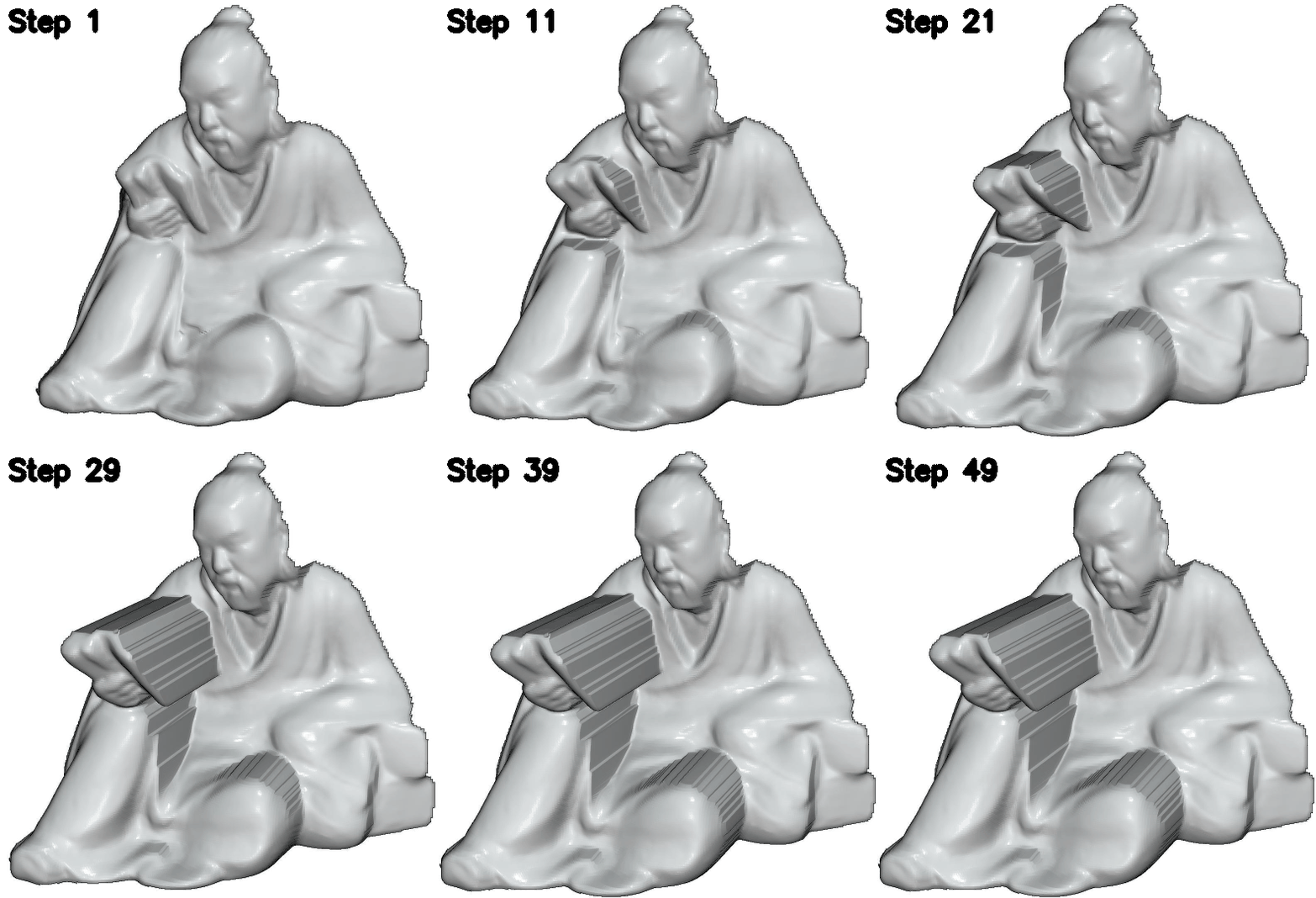
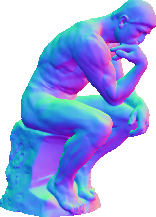
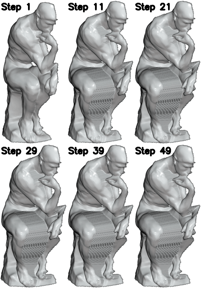
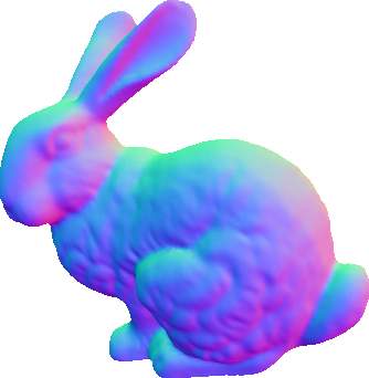
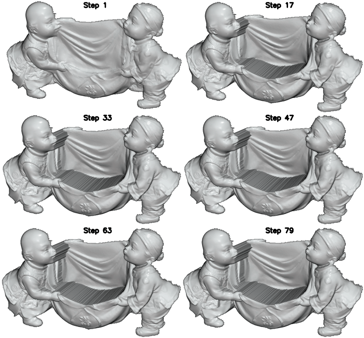
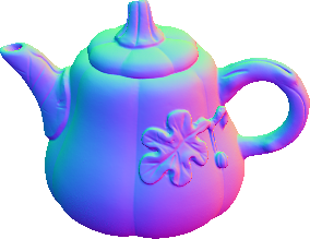
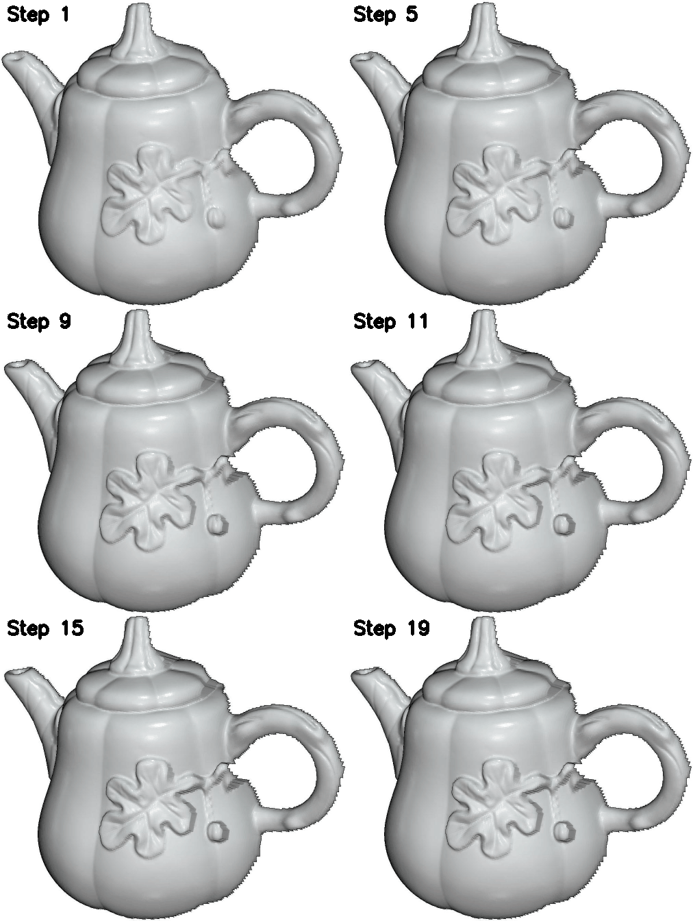
2023-11-07: Code for evaluation on the DiLiGenT dataset is available now. See this section for details.
2022-08-20: I further improved the CuPy version's efficiency but sacrificed the code's readability. Read the NumPy version first if you are interested in implementation details.
2022-08-09: A CuPy version written by Yuliang Xiu is available now. It can run on NVIDIA graphics cards and is much more efficient especially when the normal map's dimension becomes huge. The usage is the same as the NumPy version.
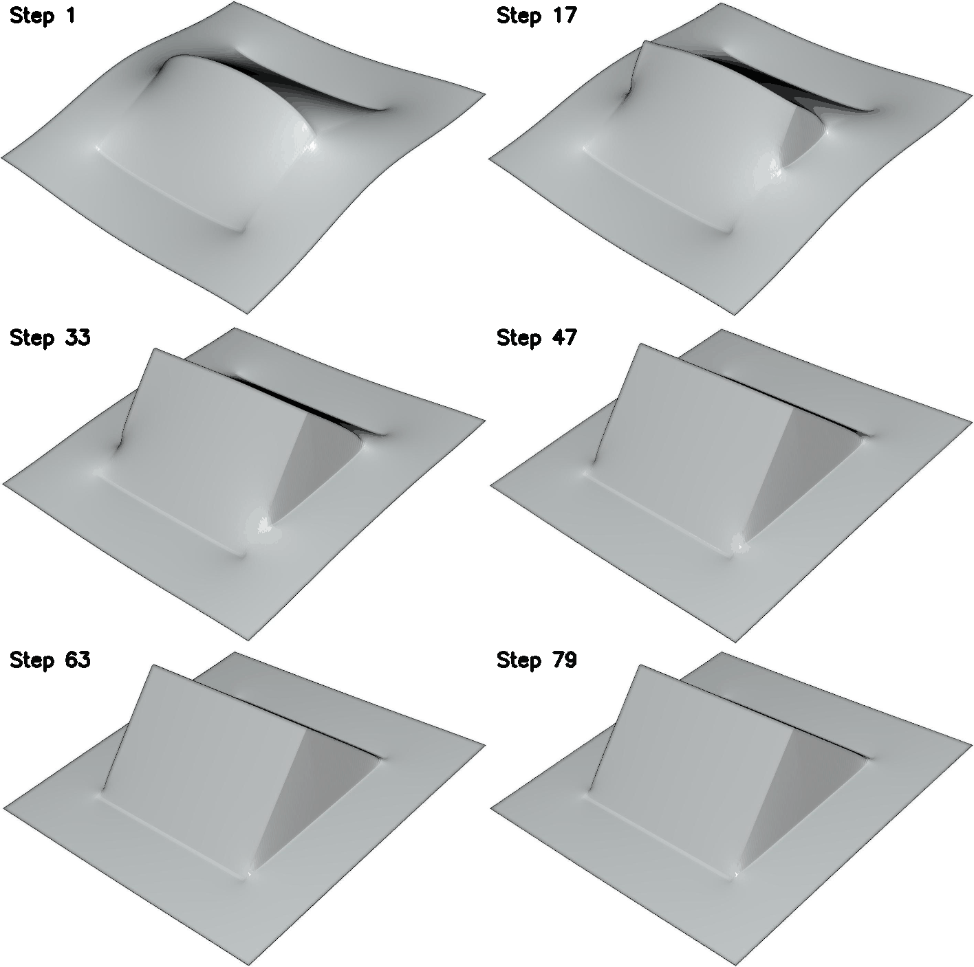
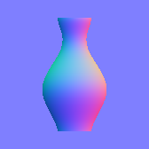
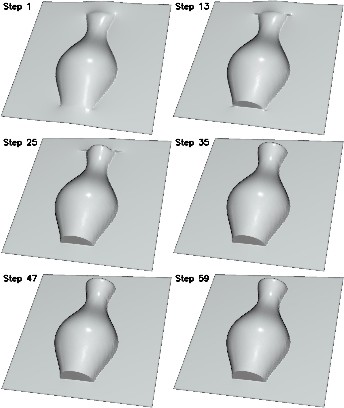
The left one is "tent," and the right one is "vase."
Normal maps rendered by Mitsuba 0.6. The left one is rendered by an orthographic camera, and the right two are by a perspective camera.
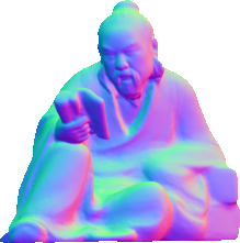
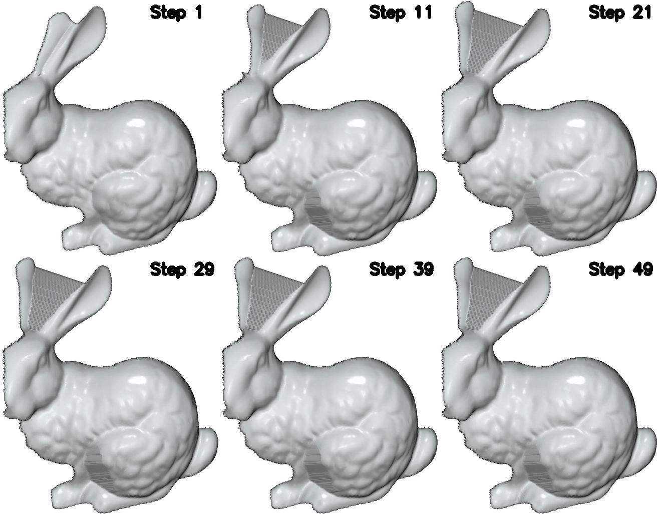
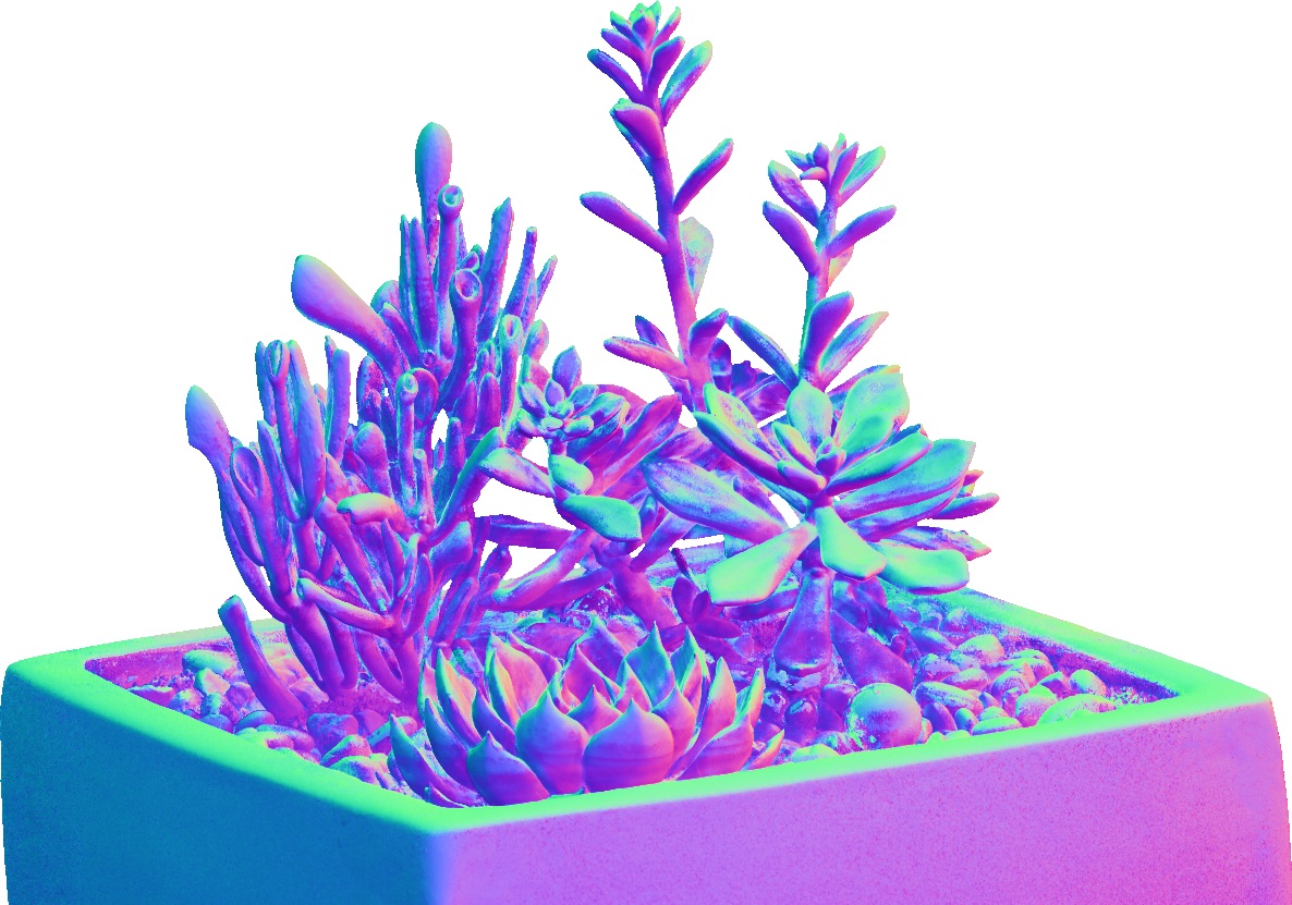
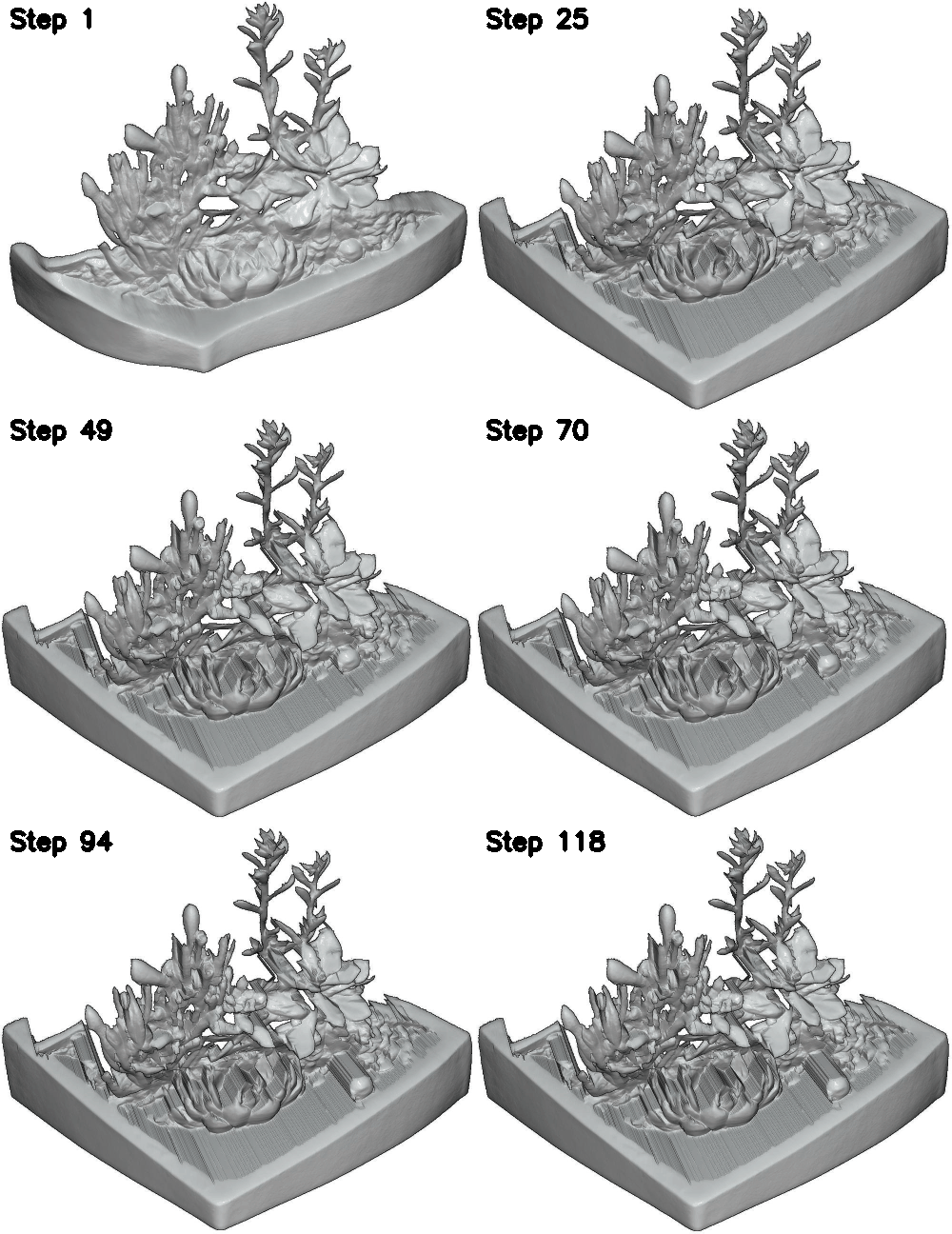
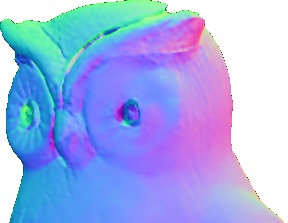
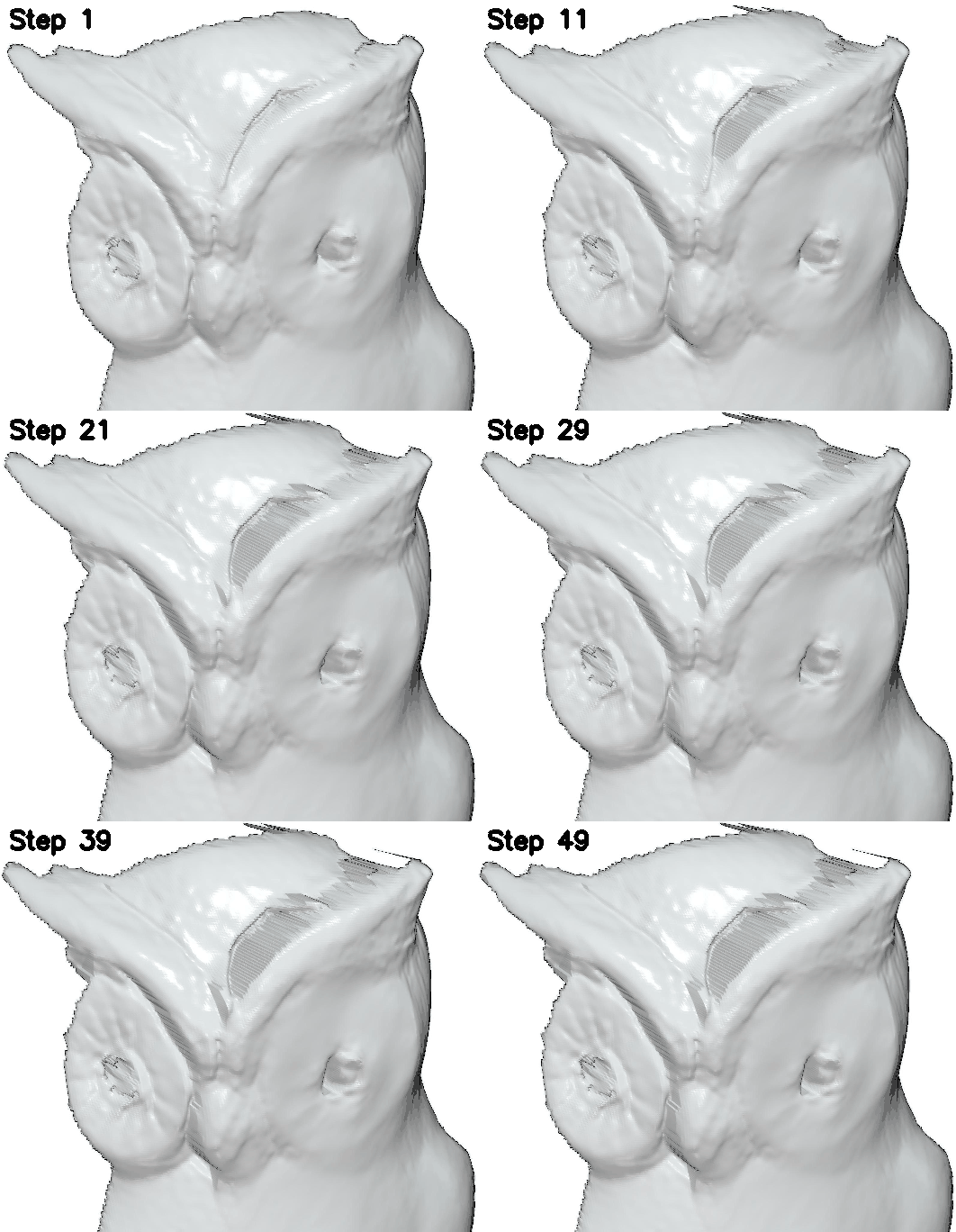
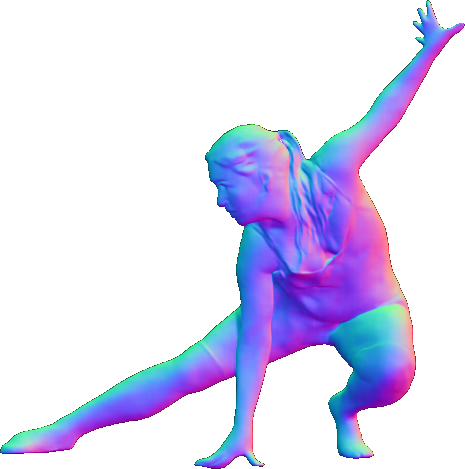
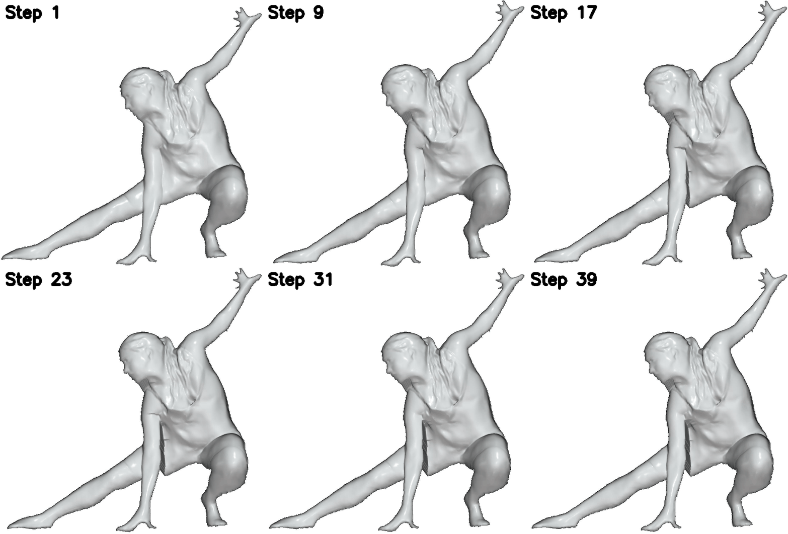
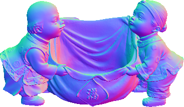
From left to right in the following, we show reconstruction results from the real-world normal maps estimated by CNN-PS, deep polarization 3D imaging, and ICON, respectively.
The following perspective normal maps are from DiLiGenT dataset.
Our implementation was tested using Python 3.7 and mainly depends on Numpy and Scipy for numerical computation, PyVista for mesh IO, and OpenCV for image IO.
You can ensure the required packages are installed in your python environment by running:
pip install -r requirements.txt
If you want to use the CuPy version on GPU, follow the official guide to install CuPy. Cuda 11.3 and cupy-cuda11x are recommended according to this issue.
The data folder contains all surfaces we used in the paper.
Each normal map and its mask are put in a distinct folder.
For the normal map in the perspective case, its folder contains an extra K.txt recording the 3x3 camera intrinsic matrix.
Our code determines the perspective or orthographic case based on whether or not there is a K.txt in the normal map's folder.
To obtain the integrated surface of a specific normal map, pass the normal map's folder path to the script bilateral_normal_integration_numpy.py.
For example,
python bilateral_normal_integration_numpy.py --path data/Fig4_reading
This script will save the integrated surface and discontinuity maps in the same folder.
The default parameter setting is k=2 (the sigmoid function's sharpness), iter=100 (the maximum iteration number of IRLS),
and tol=1e-5 (the stopping tolerance of IRLS).
You can change the parameter settings by running, for example,
python bilateral_normal_integration_numpy.py --path data/supp_vase -k 4 --iter 100 --tol 1e-5
Our setups for `k` and `iter`
| surfaces | k | iter |
|---|---|---|
| Fig. 1 the thinker | 2 | 100 |
| Fig. 4 stripes | 2 | 100 |
| Fig. 4 reading | 2 | 100 |
| Fig. 5 plant | 2 | 150 |
| Fig. 5 owl | 2 | 100 |
| Fig. 5 human | 2 | 100 |
| Fig. 6 bunny | 2 | 100 |
| Fig. 7 all DiLiGenT objects | 2 | 100 |
| supp vase | 4 | 100 |
| supp tent | 1 | 100 |
| supp limitation2 | 4 | 100 |
| supp limitation3 | 2 | 300 |
To reproduce the quantitative evaluation in Fig. 7 of our paper, first download the GT depth maps and extract it in the root directory, then run the following script:
python evaluation_diligent.py
This script reports the MADEs for DiLiGenT objects. The results are slightly better than in the paper for some objects because there may be some implementation improvements since we report the metrics in the paper.
You can test our method using your normal maps. Put the following in the same folder, and pass the folder path to the script, as abovementioned.
"normal_map.png": The RGB color-coded normal map. Check main paper's Fig. 1(a) for the coordinate system. We recommend saving the normal maps as 16-bit images to reduce the discretization error."mask.png": The integration domain should be white (1.0 or 255); the background should be black (0). If no mask is provided, the integration domain is assumed to be the entire image."K.txt"(perspective case): the (3, 3) camera intrinsic matrix. We usednp.savetxt("K.txt", K)to save the camera matrix into the txt file.
Reading the normal map from an RGB image inevitably introduces discretization errors, e.g.,
the n_x continuously defined in [-1, 1] can only take 256 or 65536 possible values in an 8-bit or 16-bit image, respectively.
If you want to avoid such error, you can directly call the function bilateral_normal_integration() in your code by
depth_map, surface, wu_map, wv_map, energy_list = bilateral_normal_integration(normal_map, mask, k=2, K=None, max_iter=100, tol=1e-5)
The key hyperparameter here is the small k. It controls how easily the discontinuity can be preserved.
The larger k is, discontinuities are easier to be preserved.
However, a very large k may introduce artifacts around discontinuities and over-segment the surface,
while a tiny k can result in smooth surfaces.
We recommend set k=2 initially (it should be fine in most cases), and tune it depending on your results.
Our ECCV paper does not discribe how to use the information from a prior depth map if it is available. We present the code here because there are people asking for this feature. Suppose you have a prior depth map recording coarse geometry information, and you want to fuse the coarse depth map with the normal map with fine geometry details. You can call our function in your code in this way:
depth_map, surface, wu_map, wv_map, energy_list = bilateral_normal_integration(normal_map,
                                                                               normal_mask,
                                                                               k=2,
                                                                               depth_map=depth_map,
                                                                               depth_mask=depth_mask,
                                                                               lambda1=1e-4,
                                                                               K=None)
Here, the normal map, normal mask, depth map, and the depth mask should be of the same dimension. But the foreground of the depth mask need not be identical to the normal mask. That is, the prior depth map can be either sparse or dense, depending on your application. The refined depth map will have the same domain as the normal map. A new hyperparameter lambda1 is introduced to control the effect of the prior depth map. The larger lambda1 is, the resultant depth map will appear closer to the prior depth map. Depth normal fusion also works in both orthographic and perspective cases.
If you find our work useful in your research, please consider citing:
@inproceedings{bini2022cao,
  title={Bilateral Normal Integration},
  author={Cao, Xu and Santo, Hiroaki and Shi, Boxin and Okura, Fumio and Matsushita, Yasuyuki},
  booktitle=ECCV,
  year={2022}
}


