NIDDL - Neuro Imaging Denoising Via Deep Learning

version is available here now with Napari denoiser.

Download using git clone -b pytorch https://github.com/shiveshc/NIDDL.git
Much easier to install and use (checkout example.ipynb).
Denoise in Napari by running napari_niddl.py

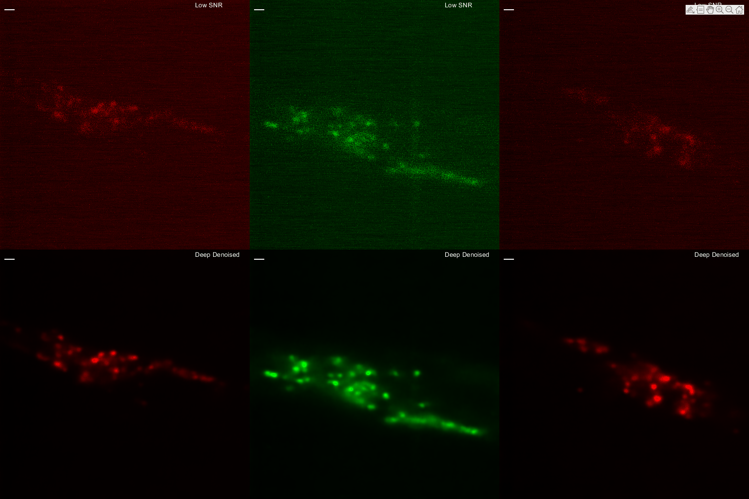
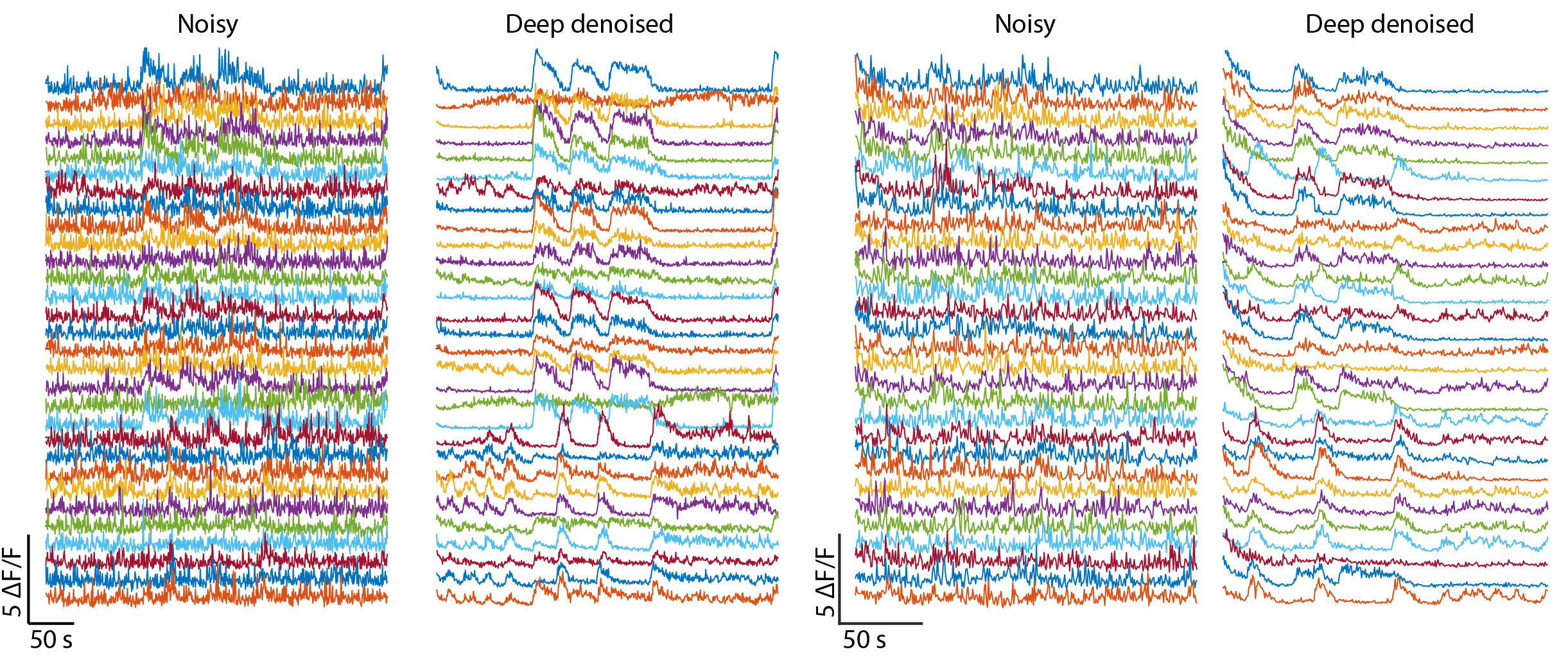
Deep denoising pushes the limit of functional data acquisition by recovering high SNR calcium traces from low SNR videos acquired using low laser power or smaller exposure time. Thus deep denoising enables faster and longer volumetric recordings. For more details, our paper is avalable.

If you find our work useful, please cite

Chaudhary, S., Moon, S. & Lu, H. Fast, efficient, and accurate neuro-imaging denoising via supervised deep learning. Nat Commun 13, 5165 (2022). https://doi.org/10.1038/s41467-022-32886-w

Denoise whole-brain videos

Denoise mechanosensory neurites

Recover high SNR calcium traces

Installation
Additional system requirements
Train on new dataset
Denoise calcium activity recordings
Denoise independent images
Run sample datasets

Installation

Installation steps tested for Windows 10 64-bit and Python 3.5

1. Download NIDDL repository

Open Git Bash terminal, navigate to desired location and clone repository using git clone https://github.com/shiveshc/NIDDL.git.

Or click on Code button on top right corner and Download ZIP.

2. Setting up venv and installing libraries

Open command line terminal as administrator and navigate to cloned repository path using cd .\NIDDL.

Next run following commands -

Windows 10	MacOS
1. `python -m venv env`	1. `python -m venv env`
2. `env\Scripts\activate.bat`	2. `source env/bin/activate`
3. `python -m pip install --upgrade "pip < 21.0"`	3. `python -m pip install --upgrade "pip < 21.0"`
4. `pip install -r requirements.txt`	4. `pip install -r requirements.txt`

Installation should take 10-15 minutes.

Common installation errors -

pip version is not upgraded
solution : upgrade pip using python -m pip install --upgrade pip
pip version is not compatible with python version
solution : install suitable pip version e.g. pip version < 21.0 is compatible with Python 3.5.

Additional system requirements

Model training using GPUs is much faster and thus preferred. To be able to use GPUs, suitable NVIDIA drivers and CUDA libraries must be installed. Additional instructions on setting up tensorflow-gpu can be found at Software requirements and Windows setup.

For tensorflow 1.6.0 currently setup in venv, CUDA v9.0 and cudnn-9.0-windows10-x64-v7.6.4.38 downloaded from cudnn archives works for Windows 10 64-bit.

Train on new dataset

To train network on new data, pairs of noisy i.e. low SNR images (acquired at low laser power or small exposure time conditions) and clean i.e. high SNR images (acquired at high laser power or long exposure time conditions) are needed. Currently supported image size is 512 x 512 x d where d is number of images in stack. For other image sizes, either resize images first or channel dimensions need to be changed in architecture files in cnn_archs folder.

Structure of training data folder should be organised as below -

data
├───gt_imgs
│   ├───img_1
│   │       z_1.tif
│   │       z_2.tif
│   │       ...
│   │
│   ├───img_2
│   │       z_1.tif
│   │       z_2.tif
│   │       ...
│   │
│   └───img_3
│           z_1.tif
│           z_2.tif
│           ...
│
└───noisy_imgs
    ├───img_1
    │       z_1.tif
    │       z_2.tif
    │       ...
    │
    ├───img_2
    │       z_1.tif
    │       z_2.tif
    │       ...
    │
    └───img_3
            z_1.tif
            z_2.tif
            ...

Run python train.py -h to see usage and input arguments. The output on terminal should look like below -

usage: train.py [-h] [-out OUT]
               [-arch {unet,unet_fixed,hourglass_wres,hourglass_wores}]
               [-mode {2D,2.5D,3D}] [-depth DEPTH] [-loss {l2,l1}]
               [-epochs EPOCHS] [-lr LR] [-bs BS] [-tsize TSIZE]
               data run {1,0}

train CNN model to denoise volumetric functional recordings

positional arguments:
 data                  training data path
 run                   run number to distinguish different runs
 {1,0}                 1 if train network on max projection of 3D stacks else
                       0

optional arguments:
 -h, --help            show this help message and exit
 -out OUT              location for saving results
 -arch {unet,unet_fixed,hourglass_wres,hourglass_wores}
                       CNN architechture to use for training (default is
                       hourglass_wres)
 -mode {2D,2.5D,3D}    training mode (default is 2D)
 -depth DEPTH          stack depth to use for training (must be odd number,
                       default is 1)
 -loss {l2,l1}         L2 or L1 loss for training (default is l1)
 -epochs EPOCHS        number of epochs to train the model for (150-200 is
                       good choice, default is 150)
 -lr LR                learning rate (default is 0.001)
 -bs BS                batch size of training (default is 6)
 -tsize TSIZE          data size (number of images) to use for training

e.g. to train the network on whole-brain data with following settings -

data path - /training_data (path should have forward slashes '/')
run number - 1
train on max-projection (e.g. ventral cord or neurite data) - 0
out path - Results (path should have forward slashes '/')
architecture - unet_fixed
training mode - 2D
loss - l1
number of training epochs - 200
batch size - 10

run following commands -

env\Scripts\activate.bat
python train.py /training_data 1 0 -out Results -arch unet_fixed -mode 2D -loss l1 -epoch 200 -bs 10

Once training is finished a folder named run_unet_fixed_l1_mp0_m2D_d1_1_[tsize] will be created in Results folder. Output files in this folder should look like below (e.g. shown for a sample run)
```
Results
└───run_unet_fixed_l1_mp0_m2D_d1_1_[tsize]
       checkpoint
       events.out.tfevents.1618996150.atl1-1-01-004-33.pace.gatech.edu
       model.data-00000-of-00001
       model.index
       model.meta
       pred_1999.png
       pred_2180.png
       pred_2227.png
       pred_2492.png
       pred_335.png
       test_data_loss.txt
       training_loss.txt
       X_1999.png
       X_2180.png
       X_2227.png
       X_2492.png
       X_335.png
       Y_1999.png
       Y_2180.png
       Y_2227.png
       Y_2492.png
       Y_335.png
```
Here -
- training_loss.txt stores epoch wise loss information on randomly sampled images from training data and test data.
- test_data_loss.txt stores loss on randomly sampled images from test data.
- checkpoint, events* and model* files will be used to restore trained weights of network to perform inference on new data.
- X*.png, Y*.png denote randomly selected noisy (input) and clean (ground-truth) images from test data. pred*.png denote corresponding denoised predictions by trained network.

Denoise calcium activity recordings

Structure of functional recording video datasets should be organised as below -

vid1
└───noisy_imgs
    ├───img_1
    │       z_1.tif
    │       z_2.tif
    │       ...
    │
    ├───img_2
    │       z_1.tif
    │       z_2.tif
    │       ...
    │
    ├───img_3
    │       z_1.tif
    │       z_2.tif
    │       ...
    ...

Here img_1, img_2 etc. can correspond to individual time-points in videos.

Run python inference.py -h to see usage and input arguments. Output on terminal should look like below -
```
usage: inference.py [-h] data [data ...] run

denoise images using weights of trained model

positional arguments:
  data        paths of datasets to be denoised
  run         path of saved trained model

optional arguments:
  -h, --help  show this help message and exit
```
e.g to denoise two video datasets with following settings -
- two video datasets with paths - /vid1, /vid2 (path should have forward slashes '/')
- save trained network path - Results/run_unet_fixed_l1_mp0_m2D_d1_1_[tsize] (path should have forward slashes '/')
run following commands -
1. env\Scripts\activate.bat
2. python inference.py /vid1 /vid2 /Results/run_unet_fixed_l1_mp0_m2D_d1_1_[tsize]
Note : to denoise max-projection calcium imaging datasets, folder structure of input dataset should remain same. In this case, use a network trained on max-projection images to denoise e.g. Results/run_hourglass_wres_l1_mp1_m2D_d1_1_[tsize] (here mp1 in run name denotes network was trained on max-projection images).
Once denoising is finished, output folders /vid1/pred_run_unet_fixed_l1_mp0_m2D_d1_1_[tsize] and /vid2/pred_run_unet_fixed_l1_mp0_m2D_d1_1_[tsize] will be created. Output files in these folders should look like below -
```
/vid1/pred_run_unet_fixed_l1_mp0_m2D_d1_1_[tsize]
│   run_unet_fixed_l1_mp0_m2D_d1_1_[tsize]_inference_runtime.txt
│
├───img_1
│       z_1.tif
│       z_2.tif
│       ...
│
├───img_2
│       z_1.tif
│       z_2.tif
│       ...
│
├───img_3
│       z_1.tif
│       z_2.tif
│       ...
...
```
Here -
- run_unet_fixed_l1_mp0_m2D_d1_1_[tsize]_inference_runtime.txt stores inference runtime information for each image.
- img_1, img_2 etc. folders store denoised images corresponding to noisy video.

Denoise independent images

E.g. to denoise 3 individual images (may be 2D images or 3D stacks) with following settings -
- 3 images with paths - data1/img_1.tif, data2/img_2.png, data2/img_3.png (path should have forward slashes '/')
- save trained network path - Results/run_unet_fixed_l1_mp0_m2D_d1_1_[tsize] (path should have forward slashes '/')
run following commands -
1. env\Scripts\activate.bat
2. python inference.py data1/img_1.tif data2/img_2.png data2/img_3.png Results/run_unet_fixed_l1_mp0_m2D_d1_1_[tsize]
Once denoising is finished, output folders data1/pred_run_unet_fixed_l1_mp0_m2D_d1_1_[tsize]_img_1.tif, data2/pred_run_unet_fixed_l1_mp0_m2D_d1_1_[tsize]_img_2.png and data2/pred_run_unet_fixed_l1_mp0_m2D_d1_1_[tsize]_img_3.png will be created. Output files in these folders should look like below -
```
data2/pred_run_unet_fixed_l1_mp0_m2D_d1_1_[tsize]_img_2.png
    run_unet_fixed_l1_mp0_m2D_d1_1_[tsize]_inference_runtime.txt
    img_2.png.tif
```
Here -
- run_unet_fixed_l1_mp0_m2D_d1_1_[tsize]_inference_runtime.txt stores inference runtime information for image.
- img_2.png.tif is the denoised output corresponding to data2/img_2.png

Run sample datasets

For demo, we provide three sample datasets, models trained for these datasets, and denoising outputs for these datasets in sample_runs folder. These datasets include -

Whole_brain - z-planes from low SNR whole-brain image stacks
Mechanosensory - max-projection images from low SNR stacks of neurites of mechanosensory neurons
VentralCord - max-projection images from low SNR stacks of motor neurons in ventral cord.

Structure of these folders looks like below (shown for \sample_runs\VentralCord) -

\sample_runs\VentralCord
│   X_101.png
│   X_109.png
│   X_11.png
│   X_115.png
│   X_118.png
│   X_122.png
│   X_123.png
│   X_26.png
│   X_42.png
│   X_67.png
│   X_76.png
│   X_81.png
│   X_91.png
│   X_92.png
│
├───run_hourglass_wres_l2_mp1_m2D_d1_2_317
│       checkpoint
│       events.out.tfevents.1625789062.atl1-1-02-006-35.pace.gatech.edu
│       model.data-00000-of-00001
│       model.index
│       model.meta
│       test_data_loss.txt
│       training_loss.txt
│
└───sample_output
    ├───pred_run_hourglass_wres_l2_mp1_m2D_d1_2_317_X_101.png
    │       run_hourglass_wres_l2_mp1_m2D_d1_2_317_inference_runtime.txt
    │       X_101.png.tif
    │
    ├───pred_run_hourglass_wres_l2_mp1_m2D_d1_2_317_X_11.png
    │       run_hourglass_wres_l2_mp1_m2D_d1_2_317_inference_runtime.txt
    │       X_11.png.tif
    │
    ├───pred_run_hourglass_wres_l2_mp1_m2D_d1_2_317_X_122.png
    │       run_hourglass_wres_l2_mp1_m2D_d1_2_317_inference_runtime.txt
    │       X_122.png.tif
    │
    ├───pred_run_hourglass_wres_l2_mp1_m2D_d1_2_317_X_42.png
    │       run_hourglass_wres_l2_mp1_m2D_d1_2_317_inference_runtime.txt
    │       X_42.png.tif
    │
    ├───pred_run_hourglass_wres_l2_mp1_m2D_d1_2_317_X_81.png
    │       run_hourglass_wres_l2_mp1_m2D_d1_2_317_inference_runtime.txt
    │       X_81.png.tif
    │
    ├───pred_run_hourglass_wres_l2_mp1_m2D_d1_2_317_X_91.png
    │       run_hourglass_wres_l2_mp1_m2D_d1_2_317_inference_runtime.txt
    │       X_91.png.tif
    │
    └───pred_run_hourglass_wres_l2_mp1_m2D_d1_2_317_X_92.png
            run_hourglass_wres_l2_mp1_m2D_d1_2_317_inference_runtime.txt
            X_92.png.tif

Here -

X_*.png correspond to low SNR images.
run_hourglass_wres_l2_mp1_m2D_d1_2_317 stores hourglass_wres cnn trained on max-projection images (mp1) from ventral cord dataset in 2D mode using l2 loss function. The stored model can be used to denoise images.
sample_output\pred_* folders store denoised outputs of trained cnn for corresponding X_*.png images.

To denoise an example image, run following commands -

env\Scripts\activate.bat
python inference.py sample_runs/VentralCord/X_26.png sample_runs/VentralCord/run_hourglass_wres_l2_mp1_m2D_d1_2_317

Upon completion, a new folder, pred_run_hourglass_wres_l2_mp1_m2D_d1_2_317_X_26.png, will be created in the same directory that contains denoised output. The folder structure should like below now -

\sample_runs\VentralCord
│   X_101.png
│   X_109.png
│   X_11.png
│   X_115.png
│   X_118.png
│   X_122.png
│   X_123.png
│   X_26.png
│   X_42.png
│   X_67.png
│   X_76.png
│   X_81.png
│   X_91.png
│   X_92.png
│
├───pred_run_hourglass_wres_l2_mp1_m2D_d1_2_317_X_26.png
│       run_hourglass_wres_l2_mp1_m2D_d1_2_317_inference_runtime.txt
│       X_26.png.tif
│
├───run_hourglass_wres_l2_mp1_m2D_d1_2_317
│       checkpoint
│       events.out.tfevents.1625789062.atl1-1-02-006-35.pace.gatech.edu
│       model.data-00000-of-00001
│       model.index
│       model.meta
│       test_data_loss.txt
│       training_loss.txt
│
└───sample_output

xusang77/NIDDL