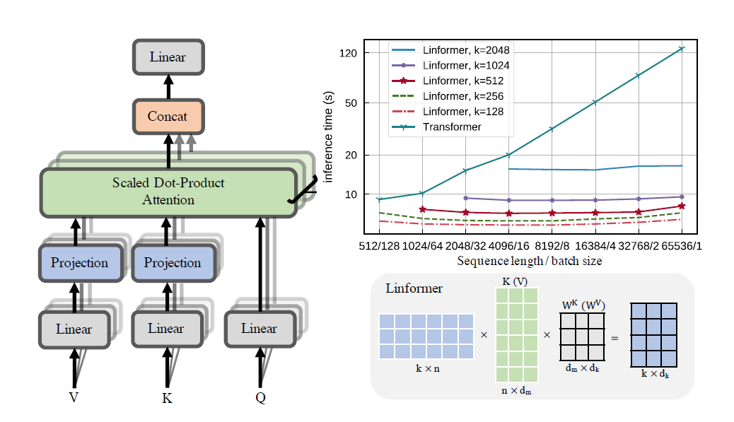
Linformer Pytorch Implementation

A practical implementation of the Linformer paper. This is attention with only linear complexity in n, allowing for very long sequence lengths (1mil+) to be attended to on modern hardware.

What is implemented so far is the encoder part of the Transformer (layers of self attention with a feed forward network), but instead of the traditional self attention, it has been replaced with the Linformer self attention, with several tuneable options.

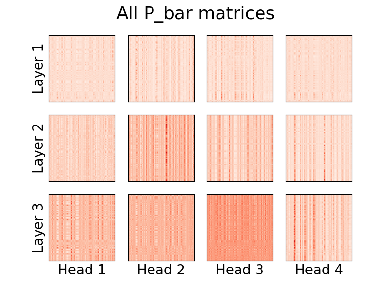
Visualization of the heads is also possible. To see more information, check out the Visualization section below.

I am not the author of the paper.

1.23m tokens

Install

pip install linformer-pytorch

Alternatively,

git clone https://github.com/tatp22/linformer-pytorch.git
cd linformer-pytorch

Code example

Linformer self attention, stacks of MHAttention and FeedForwards

from linformer_pytorch import Linformer
import torch

model = Linformer(
        input_size=262144, # Dimension 1 of the input
        channels=64, # Dimension 2 of the input
        dim_d=None, # Overwrites the inner dim of the attention heads. If None, sticks with the recommended channels // nhead, as in the "Attention is all you need" paper
        dim_k=128, # The second dimension of the P_bar matrix from the paper
        dim_ff=128, # Dimension in the feed forward network
        dropout_ff=0.15, # Dropout for feed forward network
        nhead=4, # Number of attention heads
        depth=2, # How many times to run the model
        dropout=0.1, # How much dropout to apply to P_bar after softmax
        activation="gelu", # What activation to use. Currently, only gelu and relu supported, and only on ff network.
        use_pos_emb=True, # Whether or not to use positional embeddings
        checkpoint_level="C0", # What checkpoint level to use. For more information, see below.
        parameter_sharing="layerwise", # What level of parameter sharing to use. For more information, see below.
        k_reduce_by_layer=0, # Going down `depth`, how much to reduce `dim_k` by, for the `E` and `F` matrices. Will have a minimum value of 1.
        full_attention=False, # Use full attention instead, for O(n^2) time and space complexity. Included here just for comparison
        include_ff=True, # Whether or not to include the Feed Forward layer
        w_o_intermediate_dim=None, # If not None, have 2 w_o matrices, such that instead of `dim*nead,channels`, you have `dim*nhead,w_o_int`, and `w_o_int,channels`
        ).cuda()
x = torch.randn(1, 262144, 64).cuda()
y = model(x)
print(y) # (1, 262144, 64)

Linformer Multihead attention

from linformer_pytorch import MHAttention
import torch

model = MHAttention(
        input_size=512, # Dimension 1 of the input
        channels=64, # Dimension 2 of the input
        dim=8, # Dim of each attn head
        dim_k=128, # What to sample the input length down to
        nhead=8, # Number of heads
        dropout=0, # Dropout for each of the heads
        activation="gelu", # Activation after attention has been concat'd
        checkpoint_level="C2", # If C2, checkpoint each of the heads
        parameter_sharing="layerwise", # What level of parameter sharing to do
        E_proj, F_proj, # The E and F projection matrices
        full_attention=False, # Use full attention instead
        w_o_intermediate_dim=None, # If not None, have 2 w_o matrices, such that instead of `dim*nead,channels`, you have `dim*nhead,w_o_int`, and `w_o_int,channels`
        )
x = torch.randn(1, 512, 64)
y = model(x)
print(y) # (1, 512, 64)

The Linear attention head, the novelty of the paper

from linformer_pytorch import LinearAttentionHead
import torch

model = LinearAttentionHead(
        dim=64, # Dim 2 of the input
        dropout=0.1, # Dropout of the P matrix
        E_proj, F_proj, # The E and F layers
        full_attention=False, # Use Full Attention instead
        )
x = torch.randn(1, 512, 64)
y = model(x, x, x)
print(y) # (1, 512, 64)

An easy way to get the E and F matrices can be done by calling the get_linear function. As an example, for an n of 1000 and a k of 100:

from linfromer_pytorch import get_linear
import torch

E = get_linear(1000, 100)

Checkpoint levels

As an attempt to further introduce memory savings, the concept of checkpoint levels have been introduced. The current three checkpoint levels are C0, C1, and C2. When going up checkpoint levels, one sacrifices speed for memory savings. That is, checkpoint level C0 is the fastest, but takes up the most space on the GPU, while C2 is the slowest, but takes up the least space on the GPU. The details of each checkpoint level are as follows:

C0: No checkpointing. The models runs while keeping all of the attention heads and ff layers in the GPU memory.
C1: Checkpoint each MultiHead attention as well as each ff layer. With this, increasing depth should have minimal impact on the memory.
C2: Along with the optimizations at the C1 level, checkpoint each head in each MultiHead Attention layer. With this, increasing nhead should have less of an impact on memory. However, concating the heads together with torch.cat still takes up a lot of memory, and this will hopefully be optimized out in the future.

Performance details are still unknown, but the option exists for users that want to try.

Parameter Sharing

Another attempt to introduce memory savings in the paper was to introduce parameter sharing between projections. This is mentioned in section 4 of the paper; in particular, there were 4 different types of parameter sharing that the authors discussed, and all have been implemented in this repo. The first option takes up the most memory, and each further option reduces the necessary memory requirements.

none: This is no parameter sharing. For every head and for every layer, a new E and a new F matrix is calculated for every head at each layer.
headwise: Each layer has a unique E and F matrix. All heads in the layer share this matrix.
kv: Each layer has a unique projection matrix P, and E = F = P for each layer. All heads share this projection matrix P.
layerwise: There is one projection matrix P, and every head in every layer uses E = F = P.

As started in the paper, this means that for a 12 layer, 12 head network, there would be 288, 24, 12 and 1 different projection matrices, respectively.

Note that with the k_reduce_by_layer option, the layerwise option will not be effective, since it will use the dimension of k for the first layer. Therefore, if the value of k_reduce_by_layer value is greater than 0, one should most likely not use the layerwise sharing option.

Also, note that according to the authors, in figure 3, this parameter sharing doesn't really affect the end result too much. So it may be best to just stick with layerwise sharing for everything, but the option exists for users to try it out.

Padder

One slight problem with the current implementation of the Linformer is that your sequence length has to match the input_size flag of the model. The Padder pads the input size such that the tensor can be fed into the network. An example:

from linformer_pytorch import Linformer, Padder
import torch

model = Linformer(
        input_size=512,
        channels=16,
        dim_d=32,
        dim_k=16,
        dim_ff=32,
        nhead=6,
        depth=3,
        checkpoint_level="C1",
        )
model = Padder(model)
x = torch.randn(1, 500, 16) # This does not match the input size!
y = model(x)
print(y) # (1, 500, 16)

Visualization

Starting with version 0.8.0, one can now visualize the attention heads of the linformer! To see this in action, simply import the Visualizer class, and run the plot_all_heads() function to see a picture of all the attention heads at each level, of size (n,k). Make sure that you specify visualize=True in the forward pass, as this saves the P_bar matrix so that the Visualizer class can properly visualize the head.

A working example of the code can be found below, and the same code can be found in ./examples/example_vis.py:

import torch
from linformer_pytorch import Linformer, Visualizer

model = Linformer(
        input_size=512,
        channels=16,
        dim_k=128,
        dim_ff=32,
        nhead=4,
        depth=3,
        activation="relu",
        checkpoint_level="C0",
        parameter_sharing="layerwise",
        k_reduce_by_layer=1,
        )
# One can load the model weights here
x = torch.randn(1, 512, 16) # What input you want to visualize
y = model(x, visualize=True)
vis = Visualizer(model)
vis.plot_all_heads(title="All P_bar matrices", # Change the title if you'd like
                   show=True, # Show the picture
                   save_file="./heads.png", # If not None, save the picture to a file
                   figsize=(8,6), # How big the figure should be
                   n_limit=None # If not None, limit how much from the `n` dimension to show
                   )

E and F matrices

Please upgrade to the latest version of linformer-pytorch, or a version >=0.8.0, if you downloaded it from pip! The way I calculated the E and F matrices before was that I simply used an identity matrix to downsample. However, I contacted the authors of the paper, who told me that they are actually learned parameters, and that using a nn.Linear layer with Xavier initialization is the way they used to compute these matrices.

New in version 0.8.0, a bug was discovered in the code, where the E and F matrices were of size n by d. This has been changed so it is now n by k.

Practical Tips

Note that the Linformer has O(nk) time and space complexity. So, while it may be linear in n, make sure that your k is not too large as well. These are editable with input_size and dim_k, respectively.
Speaking about k, the authors found that empirical evidence supports the fact that "the performance of Linformer model is mainly determined by the projected dimension k instead of the ratio n/k". Therefore, even when increasing sequence lengths, it may be fine to keep a relatively low, constant k (the authors showed with k=256, that it still performed almost as good as a vanilla transformer).
One more tip for k: The authors recommend that k = O(d/eps^2), if self attention wants to be approximated by full attention, with eps error.
This code, so far, is pretty much only linear layers as well as matrix multiplications. So, libraries like apex should work with this, however, in practice, it has not been tested.
In practice, I found that the memory and time requirements are more on the order of O(nkd), with n=input_size, k=dim_k, and d=dim_d.

Future work

Run some benchmark tests to see what the performance is
Instead of matrix multiplication to bring the dimensions down to k (With EKW and FVW), try to do convolution, as mentioned in the paper, with a stride length and kernel size of n/k.
Right now, all that is implemented is the encoder. Add the decoder at a future point in time.

Disclaimer

This is the first time that I am reproducing a result from a paper, so some things may be wrong. If you see a problem, please open up an issue, and I will attempt to work on it.

Thanks

Thank you to lucidrains, whose other sparse attention repositories helped me in designing this Linformer Repo.

Citations

@misc{wang2020linformer,
    title={Linformer: Self-Attention with Linear Complexity},
    author={Sinong Wang and Belinda Z. Li and Madian Khabsa and Han Fang and Hao Ma},
    year={2020},
    eprint={2006.04768},
    archivePrefix={arXiv},
    primaryClass={cs.LG}
}

@inproceedings{vaswani2017attention,
  title={Attention is all you need},
  author={Vaswani, Ashish and Shazeer, Noam and Parmar, Niki and Uszkoreit, Jakob and Jones, Llion and Gomez, Aidan N and Kaiser, {\L}ukasz and Polosukhin, Illia},
  booktitle={Advances in neural information processing systems},
  pages={5998--6008},
  year={2017}
}

"Listen with attention..."

xvr-hlt/linformer-pytorch