
pyDYNAM-O: The Dynamic Oscillation Toolbox for Python - Prerau Laboratory (sleepEEG.org)
This repository contains the updated and optimized PYTHON package code for extracting time-frequency peaks from EEG data and creating slow-oscillation power and phase histograms. The MATLAB version of DYNAM-O is available here.
Please cite the following paper when using this package:
Patrick A Stokes, Preetish Rath, Thomas Possidente, Mingjian He, Shaun Purcell, Dara S Manoach, Robert Stickgold, Michael J Prerau, Transient Oscillation Dynamics During Sleep Provide a Robust Basis for Electroencephalographic Phenotyping and Biomarker Identification, Sleep, 2022;, zsac223, https://doi.org/10.1093/sleep/zsac223
The toolbox can be referred to in the text as:
Prerau Lab's Dynamic Oscillation Toolbox (DYNAM-O) v1.0 (sleepEEG.org/)
The paper is available open access at https://doi.org/10.1093/sleep/zsac223
-
git clone <forked copy ssh url> -
Recommended conda distribution: miniconda
Apple silicon Mac: choose conda native to the ARM64 architecture instead of Intel x86
-
conda install mamba -n base -c conda-forge
cd <repo root directory with environment.yml>
mamba env create -f environment.yml
conda activate dynam_oYou may also install dynam_o in an existing environment by skipping this step.
-
cd <repo root directory with setup.py>
pip install -e .
A full description of the toolbox and tutorial can be found on the Prerau Lab site.
- Overview
- Background and Motiviation
- Quick Start
- Algorithm Summary
- Optimizations
- Repository Structure
This repository contains code to detect time-frequency peaks (TF-peaks) in a spectrogram of EEG data using the approach based on the one described in (Stokes et. al, 2022). TF-peaks represent transient oscillatory neural activity with in the EEG, which by definition will appear as a peak in the time-frequency topography of the spectrogram. Within sleep, perhaps the most important transient EEG oscillation is the sleep spindle, which has been linked to memory consolidation, and changes spindle activity have been linked with natural aging as well as numerous psychiatric and neurodegenerative disorders. This approach extracts TF-peaks by identifies salient peaks in the time-frequency topography of the spectrogram, using a method based on the watershed algorithm, which was original developed for computer vision applications. The dynamics of the TF-peaks can then be described in terms of continuous correlates of sleep depth and cortical up/down states using representations called slow-oscillation (SO) power and phase histograms. This package provides the tools for TF-peak extraction as well as the creation of the SO-power/phase histograms.
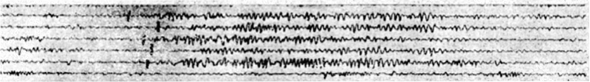
Scientists typically study brain activity during sleep using the electroencephalogram, or EEG, which measures brainwaves at the scalp. Starting in the mid 1930s, the sleep EEG was first studied by looking at the traces of brainwaves drawn on a paper tape by a machine. Many important features of sleep are still based on what people almost a century ago could most easily observe in the complex waveform traces. Even the latest machine learning and signal processing algorithms for detecting sleep waveforms are judged against their ability to recreate human observation. What then can we learn if we expand our notion of sleep brainwaves beyond what was historically easy to identify by eye?
One particularly important set of sleep brainwave events are called sleep spindles. These spindles are short oscillation waveforms, usually lasting less than 1-2 seconds, that are linked to our ability to convert short-term memories to long-term memories. Changes in spindle activity have been linked with numerous disorders such as schizophrenia, autism, and Alzheimer’s disease, as well as with natural aging. Rather than looking for spindle activity according to the historical definition, we develop a new approach to automatically extract tens of thousands of short spindle-like transient oscillation waveform events from the EEG data throughout the entire night. This approach takes advantage of the fact that transient oscillations will looks like high-power regions in the spectrogram, which represent salient time-frequency peaks (TF-peaks) in the spectrogram.
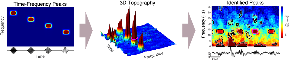
The TF-peak detection method is based on the watershed algorithm, which is commonly used in computer vision applications to segment an image into distinct objects. The watershed method treats an image as a topography and identifies the catchment basins, that is, the troughs, into which water falling on the terrain would collect.
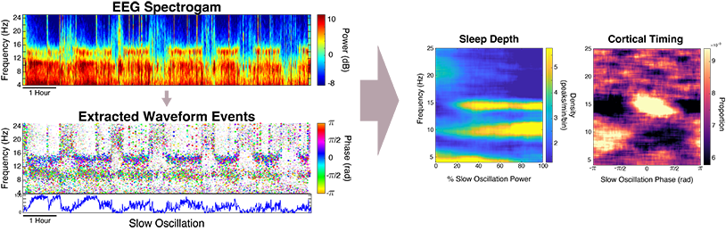
Next, instead of looking at the waveforms in terms of fixed sleep stages (i.e., Wake, REM, and non-REM stages 1-3) as di standard sleep studies, we can characterize the full continuum of gradual changes that occur in the brain during sleep. We use the slow oscillation power (SO-phase) as a metric of continuous depth of sleep, and slow-oscillation phase (SO-phase) to represent timing with respect to cortical up/down states. By characterizing TF-peak activity in terms of these two metrics, we can create graphical representations, called SO-power and SO-phase histograms. This creates a comprehensive representation of transient oscillation dynamics at different time scales, providing a highly informative new visualization technique and powerful basis for EEG phenotyping and biomarker identification in pathological states. To form the SO-power histogram, the central frequency of the TF-peak and SO-power at which the peak occured are computed. Each TF-peak is then sorted into its corresponding 2D frequency x SO-power bin and the count in each bin is normalized by the total sleep time in that SO-power bin to obtain TF-peak density in each grid bin. The same process is used to form the SO-phase histograms except the SO-phase at the time of the TF-peak is used in place of SO-power, and each row is normalized by the total peak count in the row to create probability densities.
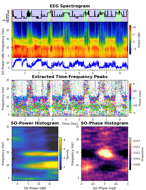
An example script is provided in the repository that takes an excerpt of a single channel of example sleep EEG data and runs the TF-peak detection watershed algorithm and the SO-power and SO-phase analyses, plotting the resulting hypnogram, spectrogram, TF-peak scatterplot, SO-power histogram, and SO-phase histogram (shown below).
After installing the package, execute the example script in an interative python console:
python -i run_example_data.pyThe following figure should be generated:
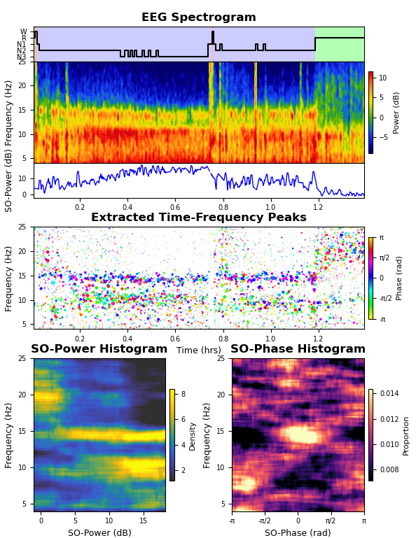
This is the general output for the algorithm. On top is the hypnogram, EEG spectrogram, and the SO-power trace. In the middle is a scatterplot of the TF-peaks with x = time, y = frequency, size = peak prominence, and color = SO-phase. On the bottom are the SO-power and SO-phase histograms.
Additionally, a peak statistics table stats_table contains features of all of the detected peaks. The example script also computes a peak_selection_inds variable, which provides the indices for just the peaks used in the SO-power/phase histograms and plotting.
These tables have the following features for each peak:
| Feature | Description | Units |
|---|---|---|
| volume | Time-frequency volume of peak in s*μV^2 | sec*μV^2 |
| peak_time | Peak time based on weighted centroid | sec |
| peak_frequency | Peak frequency based on weighted centroid | Hz |
| prominence | Peak height above baseline | μV^2/Hz |
| duration | Peak duration in seconds | sec |
| bandwidth | Peak bandwidth in Hz | Hz |
| stage | Stage: 6 = Artifact, 5 = W, 4 = R, 3 = N1, 2 = N2, 1 = N3, 0 = Unknown | Stage # |
| SOpower | Slow-oscillation power at peak time | dB |
| SOphase | Slow-oscillation phase at peak time | rad |
Once the segment has succesfully completed, you can run the full night of data by changing the following line in the example script such that the variable data_range changes from 'segment' to 'night'.
data_range = 'segment' # 'segment' vs. 'night'This should produce the following output:
For more in-depth information and documentation on the Transient Oscillation Dynamics algorithms visit the Prerau Lab website.
The following preset settings are available in our example script. As all data are different, it is essential to verify equivalency before relying on a speed-optimized solution other than precision.
- “precision”: Most accurate assessment of individual peak bounds and phase
- “fast”: Faster approach, with accurate SO-power/phase histograms, minimal difference in phase
- “draft”: Fastest approach. Good SO-power/phase histograms but with increased high-frequency peaks. Not recommended for assessment of individual peaks or precision phase estimation.
Adjust these by selecting the appropriate and changing quality from 'fast' to the appropriate quality setting.
quality = 'fast' # Quality setting 'precision','fast', or 'draft'There are also multiple normalization schemes that can be used for the SO-power.
- 'none': No normalization. The unaltered SO-power in dB.
- 'p5shift': Percentile shifted. The Nth percentile of artifact free SO-power during sleep (non-wake) times is computed and subtracted. We use the 5th percentile by default, as it roughly corresponds with aligning subjects by N1 power. This is the recommended normalization for any multi-subject comparisons.
- 'percent': %SO-power. SO-power is scaled between 1st and 99th percentile of artifact free data during sleep (non-wake) times. This this only appropriate for within-night comparisons or when it is known all subjects reach the same stage of sleep.
- 'proportional': The ratio of slow to total SO-power.
To change this, change norm_method to the appropriate value.
norm_method = 'p5shift' # Normalization of SO power 'percent','shift', or 'none'By default, the example script loads previously computed TF-peaks saved in a .csv file and only generates the SO-power and SO-phase histograms using the loaded stats_table. To run the watershed pipeline to obtain TF-peaks from scratch, change this line:
load_peaks = True # Load from csv vs computingYou can save the computed stats_table from example data by adjusting this line:
save_peaks = False # Save csv of peaks if computingThe main function to use is run_tfpeaks_soph() implemented in pipelines.py
def run_tfpeaks_soph(data, fs, stages, downsample=None, segment_dur=30, merge_thresh=8, max_merges=np.inf, trim_volume=0.8, norm_method='percent', plot_on=True):It uses the following inputs:
"""
    Parameters
    ----------
    data : ndarray
        The data to be analyzed.
    fs : int
        The sampling frequency of the data.
    stages : pandas.DataFrame
        The sleep stages of the data.
    downsample : list, optional
        The downsampling factor to be applied to the data. The default is None.
    segment_dur : int, optional
        The duration of each segment in seconds. The default is 30.
    merge_thresh : int, optional
        The minimum number of peaks that must be present in a segment for it to be considered a peak. The default is 8.
    max_merges : int, optional
        The maximum number of merges that can be performed on a segment. The default is np.inf.
    trim_volume : float, optional
        The fraction of the data to be trimmed from the beginning and end of each segment. The default is 0.8.
    norm_method : str, float, optional
        Normalization method for SO power ('percent','shift', and 'none'). The default is 'percent'.
    plot_on : bool, optional
        Whether to plot the summary figure. The default is True.
"""
The outputs are:
"""
    Returns
    -------
    stats_table : pandas.DataFrame
        A table containing the statistics.
    SOpower_hist : ndarray
        A histogram of the SO-power
    SOphase_hist : ndarray
        A histogram of the SO-phase
    SOpower_cbins : ndarray
        The SO-power bins used to compute the SO-power histogram.
    SOphase_cbins : ndarray
        The SO-phase bins used to compute the SO-phase histogram.
    freq_cbins : ndarray
        The frequency bins used to compute the SO-power/phase histograms.
    SO_power_norm : ndarray
        The normalized SO-power value.
    SO_power_times : ndarray
        The time points corresponding to each SO-power value.
    SO_phase : ndarray
        The SO-phase value.
    SO_phase_times : ndarray
        The time points corresponding to each SO-phase value.
"""For more comprehensive documentation see this tutorial on the Prerau Lab site
Here we provide a brief summary of the steps for the TF-peak detection as well as for the SO-power histogram.
Inputs: Raw EEG timeseries and Spectrogram of EEG timeseries
- Artifact Detection
- Baseline Subtraction
- Find 2nd percentile of non-artifact data and subtract from spectrogram
- Spectrogram Segmentation
- Breaks spectrogram into 30 second segments enabling parallel processing on each segment concurrently
- Extract TF-peaks for each segment (in parallel):
- Downsample high resolution segment via decimation depending on downsampling settings. Using a lower resolution version of the segment for watershed and merging allows a large runtime decrease.
- Run Matlab watershed image segmentation on lower resolution segment
- Create adjacency list for each region found from watershed
- Loop over each region and dialate slightly to find all neighboring regions
- Merge over-segmented regions to form large, distinct TF-peaks
- Calculate a merge weight for each set of neighbors
- Regions are merged iteratively starting with the largest merge weight, and affected merge weights are recalculated after each merge until all merge weights are below a set threshold.
- Interpolate TF-peak boundaries back onto high-resolution version of spectrogram segment
- Reject TF-peaks below bandwidth and duration cutoff criteria (done here to reduce number of peaks going forward to save on computation time)
- Trim all TF-peaks to 80% of their total volume
- Compute and store statistics for each peak (pixel indices, boundary indices, centroid frequency and time, amplitude, bandwidth, duration, etc.)
- Package TF-peak statistics from all segments into a single feature matrix
- Reject TF-peaks above or below bandwidth and duration cutoff criteria
Inputs: Raw EEG timeseries and TF-peak frequencies and times
- Compute SO-Power on artifact rejected EEG timeseries
- Compute multitaper spectrogram of EEG timeseries (30s windows, 15s stepsize, 29 tapers, 1Hz resolution)
- Integrate spectrogram between 0.3 and 1.5 Hz
- Normalize SO-Power via selected method
- Percent normalization: Subtracts 1st percentile and divides by 99th percentile. Used only if subjects all reach stage 3
- p5shift normalization: Subtracts 5th percentile, important for comparing across subjects
- proportion normalization: Ratio of SO-power to total power
- No normalization
- Create SO-Power and frequency bins based on desired SO-Power and frequency window and step sizes
- Compute TF-peak rate in each pixel of SO-Power-Frequency histogram
- Count how many TF-peaks fall into each pixel's given frequency and SO-Power bin
- Divide by total sleep time spent in the given SO-Power bin
Inputs: Raw EEG timeseries and TF-peak frequencies and times
- Compute SO-Phase on 0.3-1.5Hz bandpassed EEG timeseries
- Compute Herbert transform of bandpassed signal
- Unwrap Herbert phase (so that it is in terms of cumulative radians)
- Interpolate phase at each TF-peak time
- Rewrap phase of each TF-peak so that 0 radians corresponds to SO peak and -pi or pi corresponds to SO trough
- Create SO-Phase and frequency bins based on desired SO-Phase and frequency window and step sizes
- Compute TF-peak rate in each pixel of SO-Phase-Frequency histogram
- Count how many TF-peaks fall into each pixel's given frequency and SO-Phase bin
- Divide by total sleep time spent in the given SO-Phase bin
- Normalize each frequency row of histogram so that row integration adds to 1
This code is an optimized version of what was used in Stokes et. al., 2022. The following is a list of the changes made during optimization. The original unoptimized paper code can be found here.
- Candidate TF-Peak regions that are below the duration and bandwidth cutoffs are now removed prior to trimming and peak property calculations
- Empty regions that come out of the merge procedure are now removed prior to trimming and peak property calculations
- Watershed and the merging procedure now run on a lower resolution spectrogram (downsampled from the input spectrogram using decimation) to get the rough watershed regions, which are then mapped back onto the high-resolution spectrogram, from which trimming and peak property calculations are done.
- Spectrogram segment size reduced from 60s to 30s
- During the merging process, the adjacency list is now stored as unidirectional graph (instead of bidirectional), and only the larger of the merging weights between two regions is stored during iterative merge weight computation.
The contents of the "package" folder is organized as follows, with key functions:
.REPO_ROOT
├── examples/  CONTAINS EXAMPLE DATA AND EXAMPLE SCRIPT
│   ├── run_example_data.py:         Quick start example, computes the SO-Power and SO-Phase histograms, and
│   │                                 plots a summary figure. Uses example data contained in example_data folder.
│   └── _example_data/:              Example data files and saved pre-computed peaks
└── dynam_o/   MAIN PACKAGE FOLDER
    ├── multitaper.py
    │         - Multitaper spetrogram computation
    ├── SOPH.py
    │         - Functions used to compute SO-power and SO-phase histograms
    ├── TFpeaks.py
    │         - Functions used to run the watershed pipeline on a given spectrogram,
    │           including baseline removal, image segmentation, peak merging, trimming, and statistics.
    ├── utils.py
    │         - Contains various utility functions for spectral estimation and plotting
    └── pipelines.py
              - compute_tfpeaks(): Top level function to run the watershed pipeline to extract TF-peaks
              - compute_sophs(): Top level function to obtain SO-power and SO-phase histograms
              - run_tfpeaks_soph(): Main function to use for analyzing new data;
                                    calls compute_tfpeaks() and compute_sophs() internally.