Official implementation: Deep vanishing point detection: Geometric priors make dataset variations vanish, CVPR'22
Yancong Lin, Ruben Wiersma, Silvia Laura Pintea, Klaus Hildebrandt, Elmar Eisemann and Jan C. van Gemert
E-mail: yancong.linATtudelftDOTnl; r.t.wiersmaATtudelftDOTnl
Joint work from Computer Vision Lab and Computer Graphics and Visualization
Delft University of Technology, The Netherlands
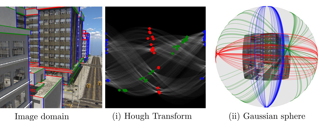
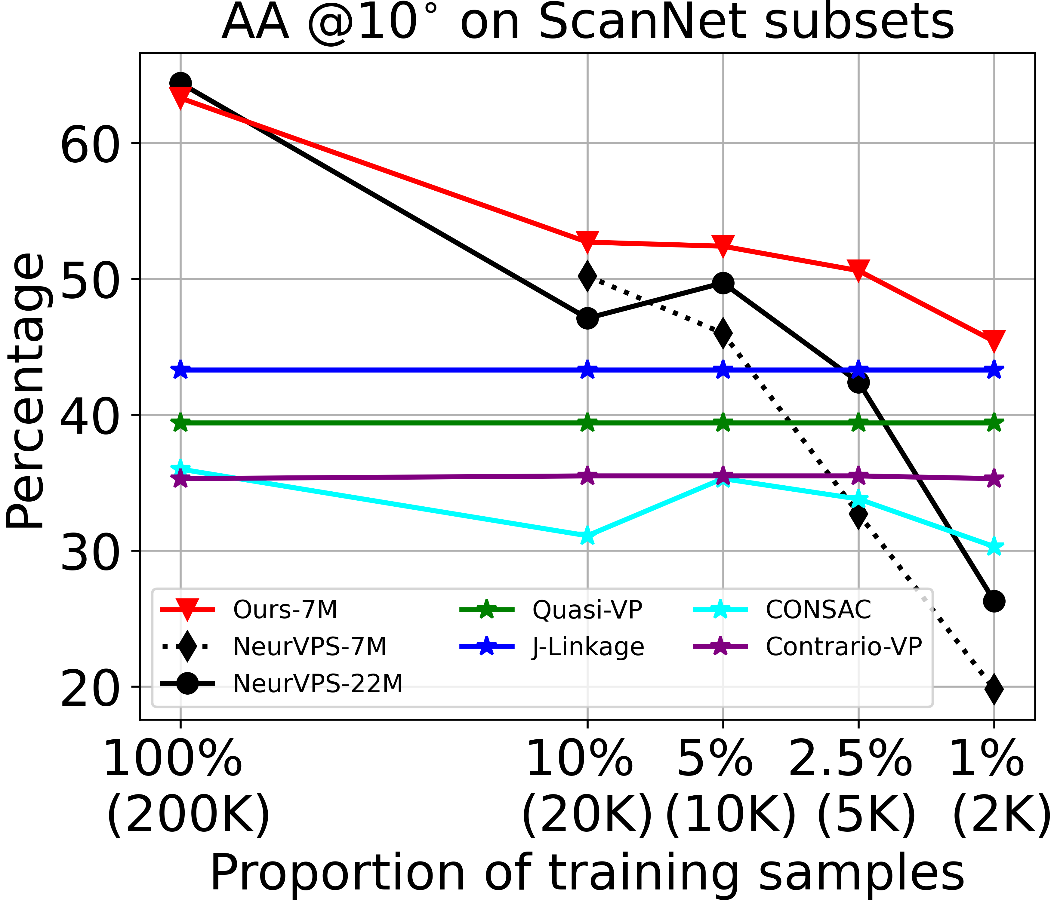
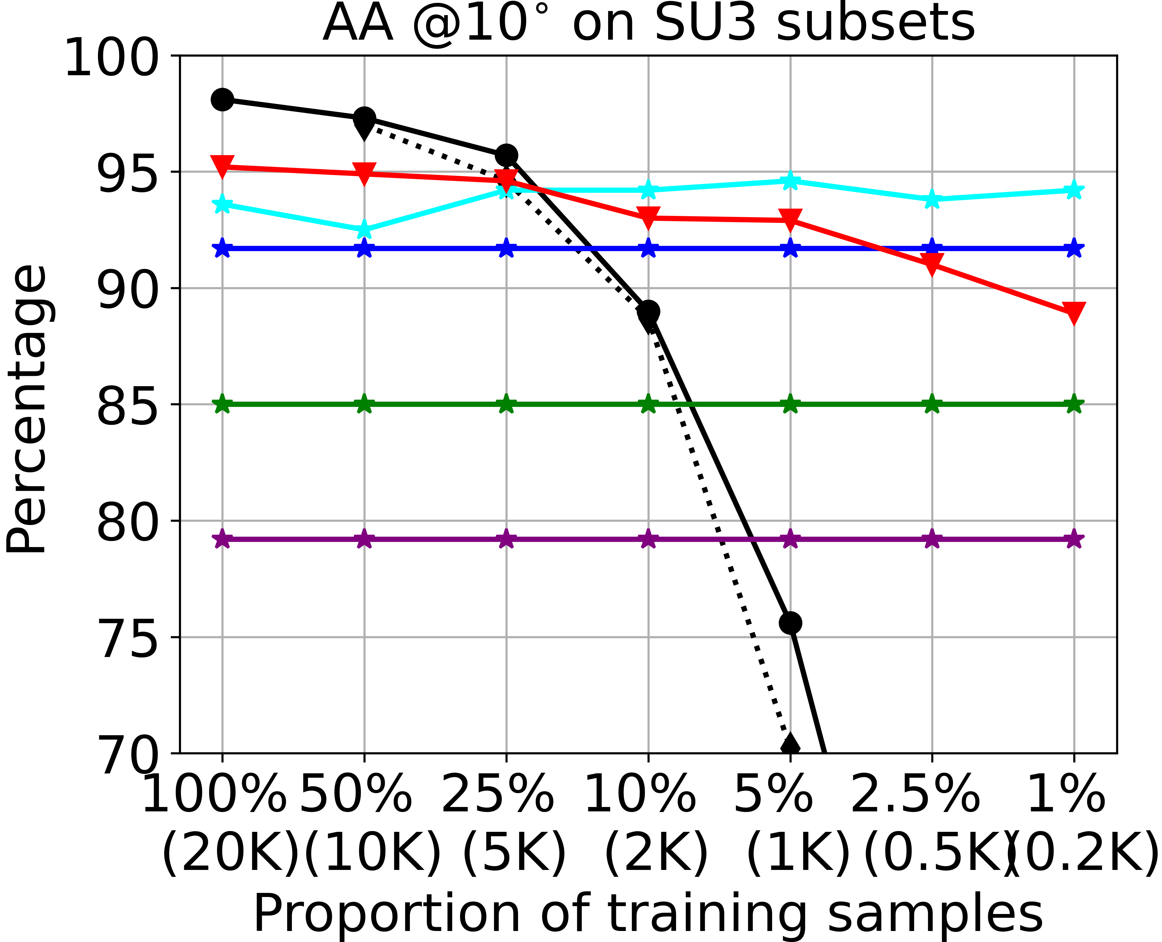
Deep learning has greatly improved vanishing point detection in images. Yet, deep networks require expensive annotated datasets trained on costly hardware and do not generalize to even slightly different domains and minor problem variants. Here, we address these issues by injecting deep vanishing point detection networks with prior knowledge. This prior knowledge no longer needs to be learned from data, saving valuable annotation efforts and compute, unlocking realistic few-sample scenarios, and reducing the impact of domain changes. Moreover, because priors are interpretable, it is easier to adapt deep networks to minor problem variations such as switching between Manhattan and non-Manhattan worlds. We incorporate two end-to-end trainable geometric priors: (i) Hough Transform -- mapping image pixels to straight lines, and (ii) Gaussian sphere -- mapping lines to great circles whose intersections denote vanishing points. Experimentally, we ablate our choices and show comparable accuracy as existing models in the large-data setting. We then validate that our model improves data efficiency, is robust to domain changes, and can easily be adapted to a non-Manhattan setting.
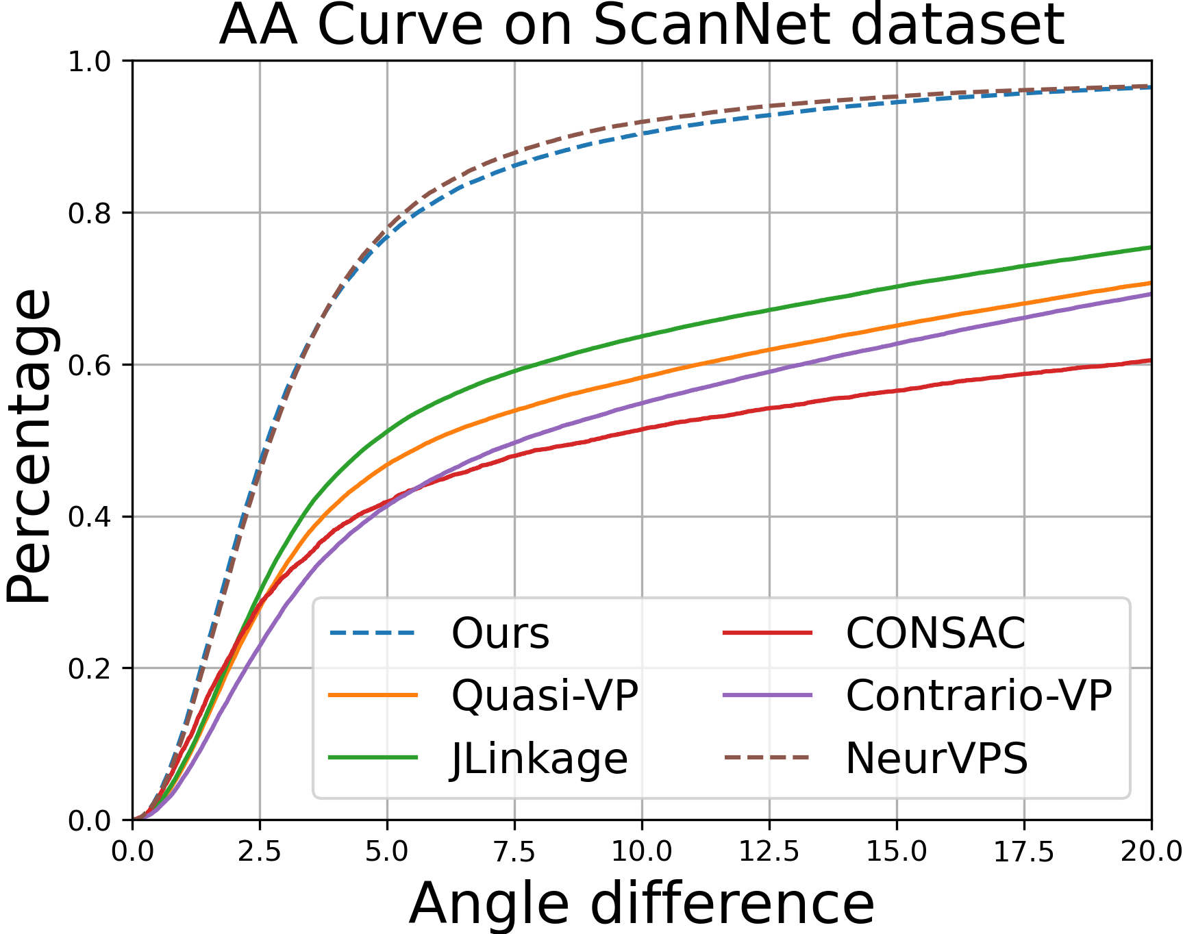
An overview of our model for vanishing point detection, with two geometric priors.(i) Competitive results on large-scale Manhattan datasets: SU3/ScanNet;
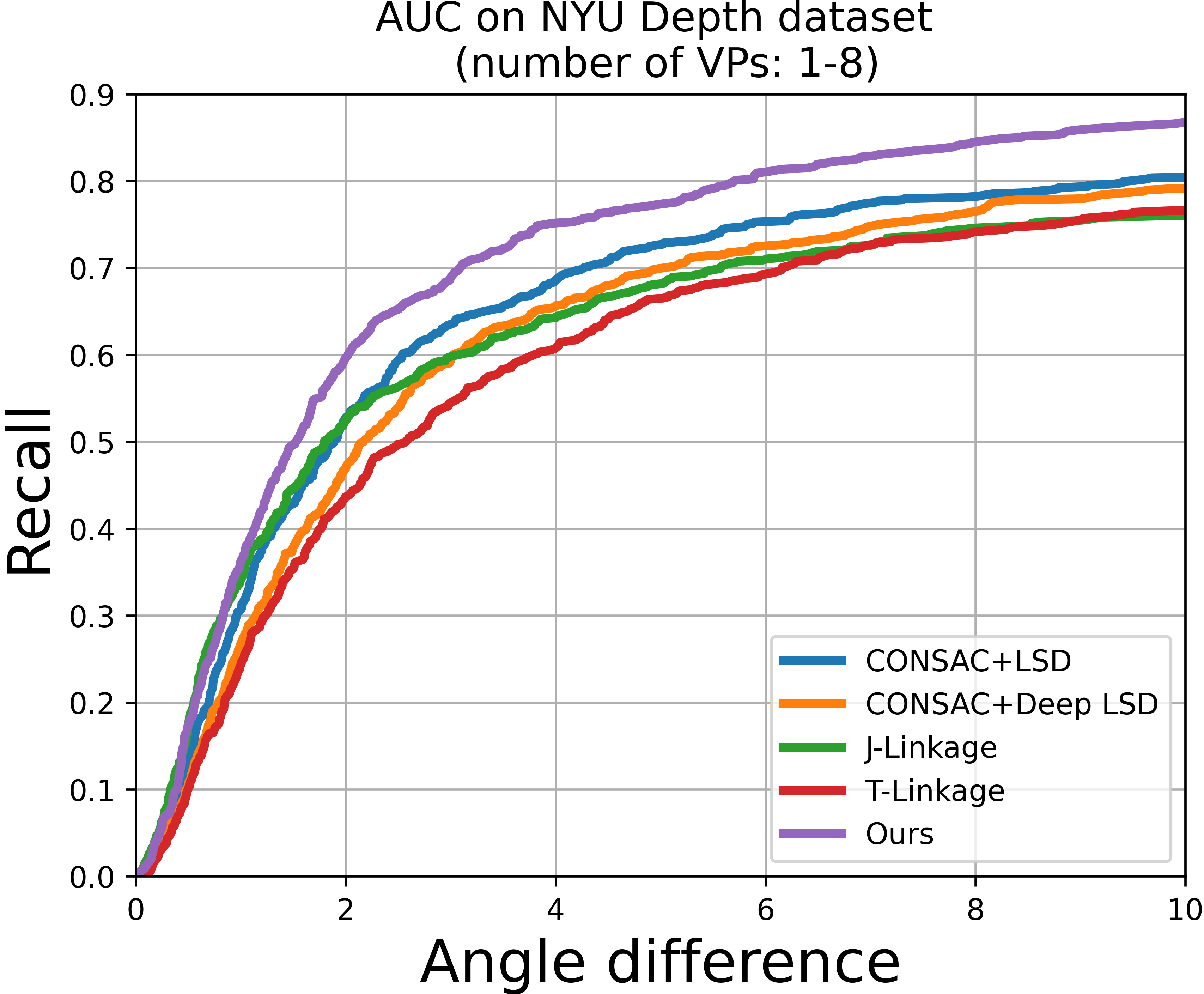
(ii) Advantage in detecting a varying number of VPs in non-Manhattan world: NYU Depth;
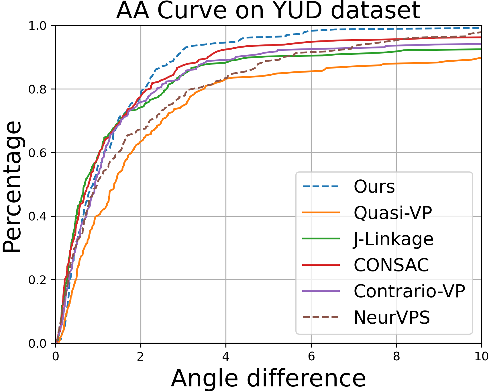
(iii) Excellent performance on new datasets, e.g. train on SU3 (synthetic)/ test on YUD (real-world).
We made necessary changes on top of NeurVPS to fit our design. Many thanks to Yichao Zhou for releasing the code.
Install miniconda (or anaconda) before executing the following commands. Our code has been tested with miniconda/3.9, CUDA/10.2 and devtoolset/6.
conda create -y -n vpd
conda activate vpd
conda env update --file config/environment.ymlSU3/ScanNet: we follow NeurVPS to process the data.
cd data
../misc/gdrive-download.sh 1yRwLv28ozRvjsf9wGwAqzya1xFZ5wYET su3.tar.xz
../misc/gdrive-download.sh 1y_O9PxZhJ_Ml297FgoWMBLvjC1BvTs9A scannet.tar.xz
tar xf su3.tar.xz
tar xf tmm17.tar.xz
tar xf scannet.tar.xz
rm *.tar.xz
cd ..
NYU/YUD: we download the data from CONSAC; and then process the data.
python dataset/nyu_process.py --data_dir path/to/data --save_dir path/to/processed_data --mat_file path/to/nyu_depth_v2_labeled.mat
python dataset/yud_process.py --data_dir path/to/data --save_dir path/to/processed_dataCompute the mapping from pixels -HT bins - Spherical points. We use GPUs (Pytorch) to speed up the calculation (~4 hours).
python parameterization.py --save_dir=parameterization/nyu/ --focal_length=1.0 --rows=240 --cols=320 --num_samples=1024 --num_points=32768 # NYU as an exampleTip: you can also download our pre-calculated parameterizations from SURFdrive.
We conducted all experiments on either GTX 1080Ti or RTX 2080Ti GPUs.
To train the neural network on GPU 0 (specified by -d 0) with the default parameters, execute
python train.py -d 0 --identifier baseline config/nyu.yamlManhattan world (3-orthogonal VPs):
python eval_manhattan.py -d 0 -o path/to/resut.npz path/to/config.yaml path/to/checkpoint.pth.tarNon-Manhattan world (unknown number of VPs, one extra step - use DBSCAN to cluster VPs on the hemisphere):
python eval_nyu.py -d 0  --dump path/to/result_folder  config/nyu.yaml  path/to/nyu/checkpoint.pth.tar
python cluster_nyu.py --datadir path/to/nyu/data --pred_dir path/to/result_folder
You can also download our checkpoints/results/logs from SURFdrive.
As an example, we use the pretrained model on NYU to detect VPs from image "example_yud.jpg". We visualize predictions (both VPs and the Gasussian sphere) in "pred.png". In this example, we do clustering on the hemisphere to detect multiple VPs.
python demo.py -d 0 config/nyu.yaml path/to/nyu/checkpoint_latest.pth.tar figs/example_yud.jpgThe pre-calculated mapping needs further exaplaination.
Please check the multi_scale branch.
The focal length in our code is in the unit of 2/max(h, w) pixel (where h, w are image height/width). Knowing focal length is a strongh prior as one can utilize the Manhattan assumption to find orthogonal VPs in the camera space. Given a focal length, you can use to_pixel to back-project a VP on the image plane.
In this case, you can set the focal length to 1.0 as in config/nyu.yaml. You might have to think about how to find VPs without the Manhattan assumption. One simple solution could be simply picking up the top-k VPs, assuming they are more or less equally spread over the hemisphere (similar to topk_orthogonal_vps). A second (better) solution is clustering as shown on the NYU dataset. There are other solutions as well. The best solution might differ from case to case.
Quantization details in this repo (Pixels - HT -Gaussian Sphere) are:
SU3 (Ours*): 128x128 - 184x180 - 32768; (Multi-Scale version, as in the paper)
SU3 (Ours): 256x256 - 365x180 - 32768;
ScanNet (Ours): 256x256 - 365x180 - 16384;
NYU/YUD (Ours): 240x320 - 403x180 - 32768;
Tab 1&2 show that quantization at 128x128 is already sufficient for a decent result. Moreover training/inference time decreases significantly. However, quantization has always been a weakness for the classic HT/Gaussian sphere, despite of their excelllence in adding inductive knowledge.
To reproduce the cross-dataset result, please refer to this issue for details.
Unfortunately, I do not have such an implementation yet at this moment.
J/T-Linkage; J-Linkage; Contrario-VP; NeurVPS; CONSAC; VaPiD?;
If you find our paper useful in your research, please consider citing:
@article{lin2022vpd,
  title={Deep vanishing point detection: Geometric priors make dataset variations vanish},
  author={Lin, Yancong and Wiersma, Ruben and and Pintea, Silvia L and Hildebrandt, Klaus and Eisemann, Elmar and van Gemert, Jan C},
  booktitle={Proceedings of the IEEE/CVF Conference on Computer Vision and Pattern Recognition (CVPR)},
  year={2022}
}