Advanced Lane Finding Project
The goals / steps of this project are the following:
- Compute the camera calibration matrix and distortion coefficients given a set of chessboard images.
- Apply a distortion correction to raw images.
- Use color transforms, gradients, etc., to create a thresholded binary image.
- Apply a perspective transform to rectify binary image ("birds-eye view").
- Detect lane pixels and fit to find the lane boundary.
- Determine the curvature of the lane and vehicle position with respect to center.
- Warp the detected lane boundaries back onto the original image.
- Output visual display of the lane boundaries and numerical estimation of lane curvature and vehicle position.
Rubric Points
Here I will consider the rubric points individually and describe how I addressed each point in my implementation.
1. Provide a Writeup / README that includes all the rubric points and how you addressed each one. You can submit your writeup as markdown or pdf. Here is a template writeup for this project you can use as a guide and a starting point.
You're reading it!
1. Briefly state how you computed the camera matrix and distortion coefficients. Provide an example of a distortion corrected calibration image.
The code for this step is contained in the section of 2 Calculate Camera Calibration Matrix and Distortion Coefficients in P4.ipynb
def find_object_image_sets(path_str, nx, ny, show_img=False):
    object_sets = []
    image_sets = []

    # Generate a matrics, have nx * ny rows, 3 colomns, type is np.float32
    object_points = np.zeros((nx * ny, 3), np.float32)
    object_points[:, :2] = np.mgrid[0:nx, 0:ny].T.reshape(-1, 2)

    # Load all chessboard images path
    chessboard_imgs_path = glob.glob(path_str)

    for chessboard_img_path in chessboard_imgs_path:
        # Load image
        img = cv2.imread(chessboard_img_path)

        # Convert into grayscale
        gray = cv2.cvtColor(img, cv2.COLOR_BGR2GRAY)

        ret, corners = cv2.findChessboardCorners(gray, (nx, ny), None)

        if ret == True:
            object_sets.append(object_points)
            image_sets.append(corners)

            # Draw the corners on the chessboard
            if show_img == True:
                cv2.drawChessboardCorners(img, (nx, ny), corners, ret)
                f, ax = plt.subplots(1, 1, figsize=(7, 7))
                ax.imshow(img)
                ax.axis('off')
                ax.set_title(chessboard_img_path, fontsize = 20)

    size = (mpimg.imread(chessboard_imgs_path[0]).shape[1], mpimg.imread(chessboard_imgs_path[0]).shape[0])

    ret, mtx, dist, rvecs, tvecs = cv2.calibrateCamera(object_sets, image_sets, size, None, None)
    return (mtx, dist)
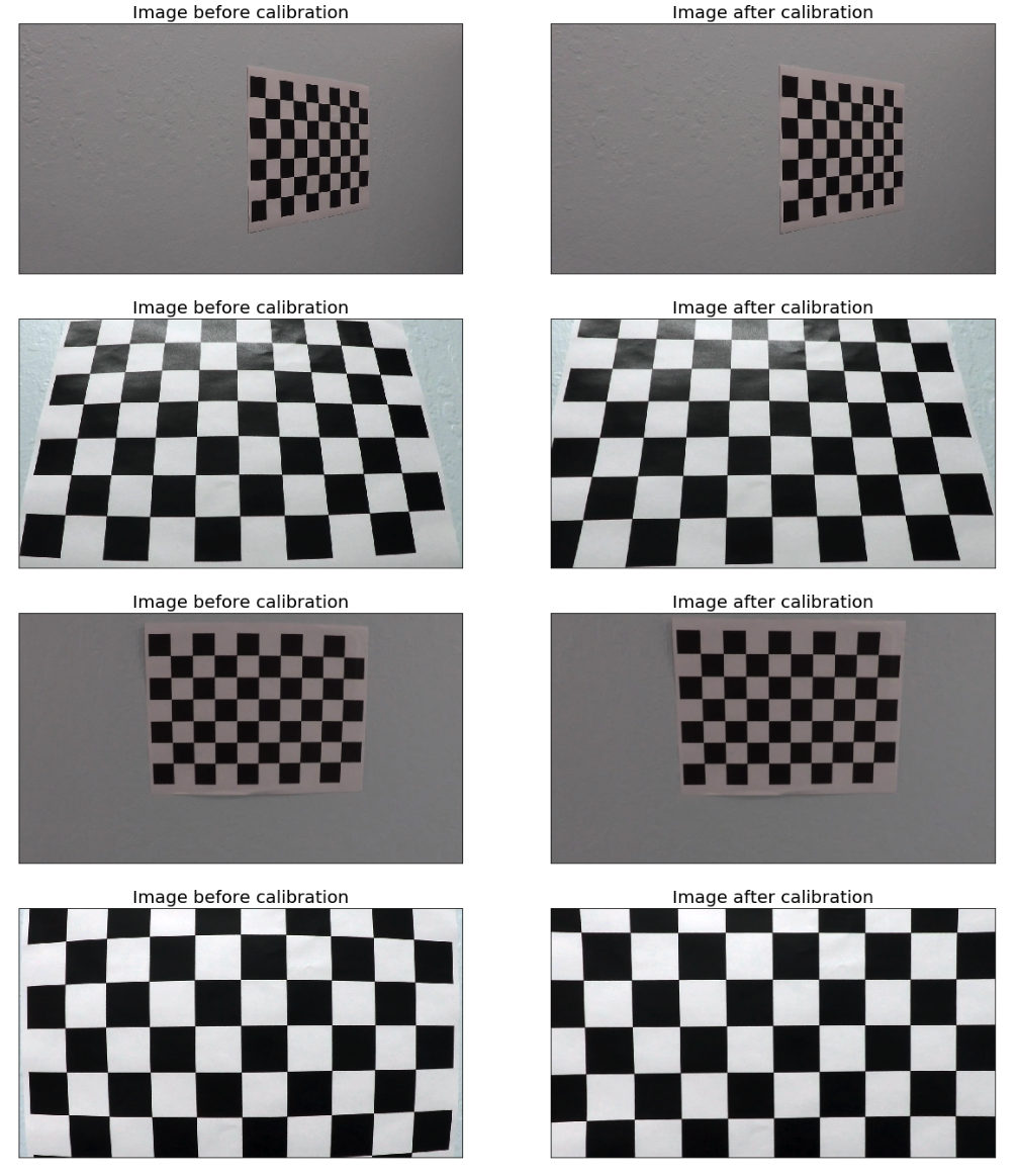
I start by preparing "object points", which will be the (x, y, z) coordinates of the chessboard corners in the world. Here I am assuming the chessboard is fixed on the (x, y) plane at z=0, such that the object points are the same for each calibration image. Thus, object_points is just a replicated array of coordinates, and object_sets will be appended with a copy of it(object_points) every time I successfully detect all chessboard corners in a test image. image_sets will be appended with the (x, y) pixel position of each of the corners in the image plane with each successful chessboard detection. The corners is detected by cv2.findChessboardCorners(). Here are some outcome of using cv2.findChessboardCorners() to find the corner:
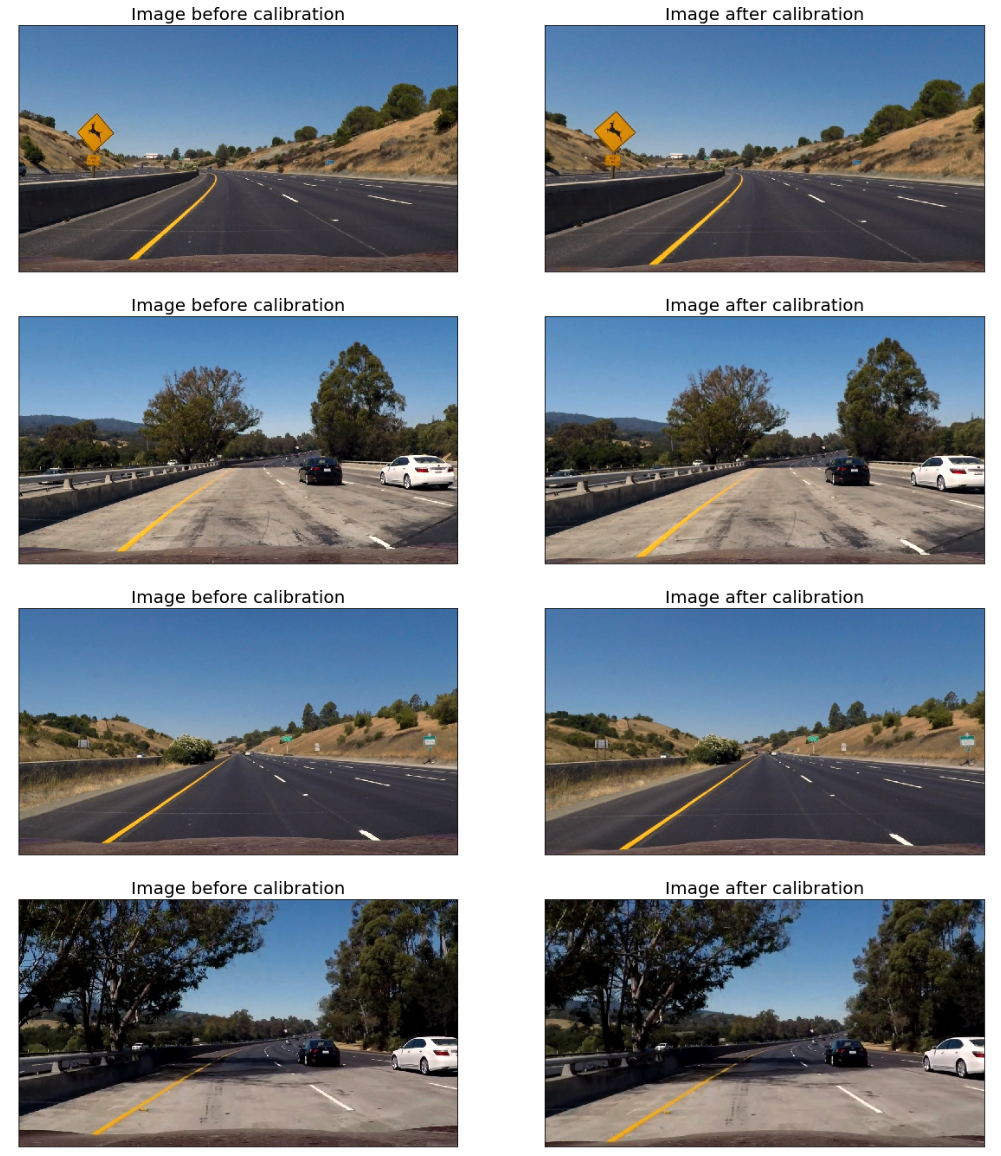
I then used the output object_sets and image_sets to compute the camera calibration and distortion coefficients using the cv2.calibrateCamera() function. I applied this distortion correction to the test image using the cv2.undistort() function and obtained this result:
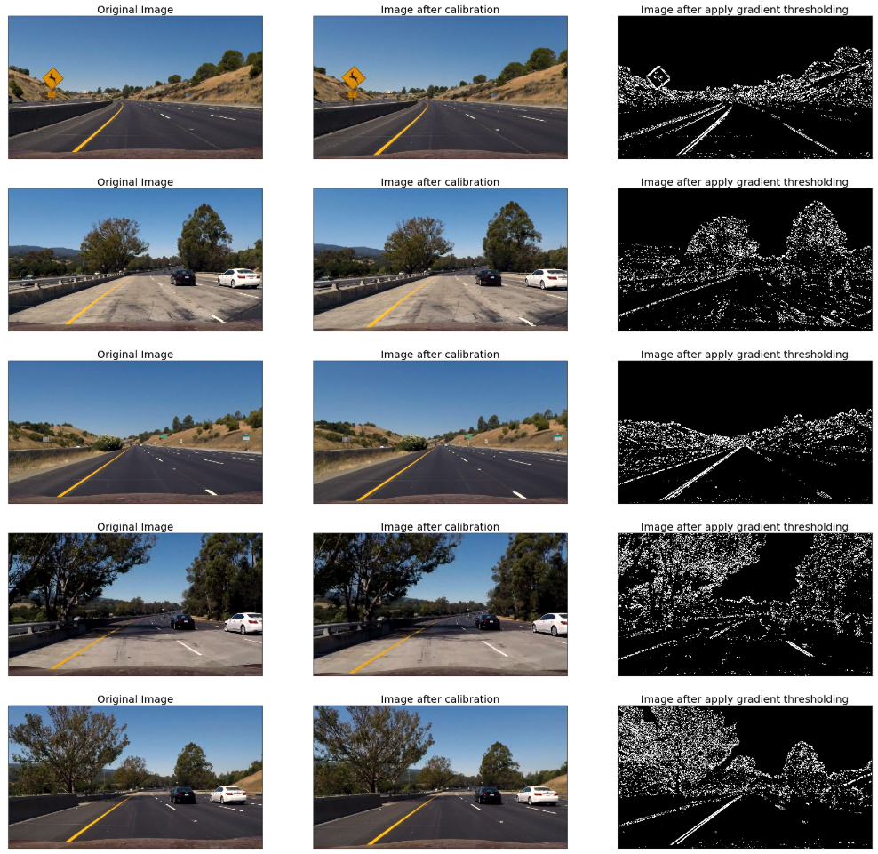
To demonstrate this step, I will describe how I apply the distortion correction to some of the test images like this:
2. Describe how (and identify where in your code) you used color transforms, gradients or other methods to create a thresholded binary image. Provide an example of a binary image result.
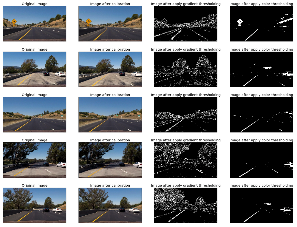
I used a combination of color and gradient thresholds to generate a binary image (thresholding steps at section 4 Color & Gradient Thresholding).
- Sober Operation
def abs_sobel_thresh(img, orient='x', thresh=(0,255)):
    # Convert to grayscale
    gray = cv2.cvtColor(img, cv2.COLOR_RGB2GRAY)
    # Apply x or y gradient with the OpenCV Sobel() function
    # and take the absolute value
    if orient == 'x':
        abs_sobel = np.absolute(cv2.Sobel(gray, cv2.CV_64F, 1, 0))
    if orient == 'y':
        abs_sobel = np.absolute(cv2.Sobel(gray, cv2.CV_64F, 0, 1))
    # Rescale back to 8 bit integer
    scaled_sobel = np.uint8(255*abs_sobel/np.max(abs_sobel))
    # Create a copy and apply the threshold
    binary_output = np.zeros_like(scaled_sobel)
    # Here I'm using inclusive (>=, <=) thresholds, but exclusive is ok too
    binary_output[(scaled_sobel >= thresh[0]) & (scaled_sobel <= thresh[1])] = 1

    # Return the result
return binary_output- Magnitude of Gradient Thresholding
def mag_thresh(img, sobel_kernel=3, mag_thresh=(0, 255)):
    # Convert to grayscale
    gray = cv2.cvtColor(img, cv2.COLOR_RGB2GRAY)
    # Take both Sobel x and y gradients
    sobelx = cv2.Sobel(gray, cv2.CV_64F, 1, 0, ksize=sobel_kernel)
    sobely = cv2.Sobel(gray, cv2.CV_64F, 0, 1, ksize=sobel_kernel)
    # Calculate the gradient magnitude
    gradmag = np.sqrt(sobelx**2 + sobely**2)
    # Rescale to 8 bit
    scale_factor = np.max(gradmag)/255
    gradmag = (gradmag/scale_factor).astype(np.uint8)
    # Create a binary image of ones where threshold is met, zeros otherwise
    binary_output = np.zeros_like(gradmag)
    binary_output[(gradmag >= mag_thresh[0]) & (gradmag <= mag_thresh[1])] = 1

    # Return the binary image
return binary_output- Direction of Gradient Thresholding
def dir_threshold(img, sobel_kernel=3, thresh=(0, np.pi/2)):
    # Grayscale
    gray = cv2.cvtColor(img, cv2.COLOR_RGB2GRAY)
    # Calculate the x and y gradients
    sobelx = cv2.Sobel(gray, cv2.CV_64F, 1, 0, ksize=sobel_kernel)
    sobely = cv2.Sobel(gray, cv2.CV_64F, 0, 1, ksize=sobel_kernel)
    # Take the absolute value of the gradient direction,
    # apply a threshold, and create a binary image result
    absgraddir = np.arctan2(np.absolute(sobely), np.absolute(sobelx))
    binary_output =  np.zeros_like(absgraddir)
    binary_output[(absgraddir >= thresh[0]) & (absgraddir <= thresh[1])] = 1

    # Return the binary image
return binary_output- Combination of Sober/Magnitude/Direction Gradient Thresholding
def gradient_threshold(img, ksize=15, sthresh=(20, 100), mthresh =(20, 100), dthresh=(0.7, 1.3)):
    gradx = abs_sobel_thresh(img, orient='x', thresh=sthresh)
    grady = abs_sobel_thresh(img, orient='y', thresh=sthresh)
    mag_binary = mag_thresh(img, sobel_kernel=ksize, mag_thresh=mthresh)
    dir_binary = dir_threshold(img, sobel_kernel=ksize, thresh=dthresh)

    combined_binary = np.zeros_like(dir_binary)
    combined_binary[((gradx == 1) & (grady == 1)) | ((mag_binary == 1) & (dir_binary == 1))] = 1

    return combined_binary
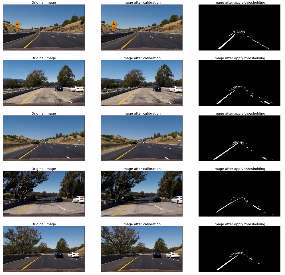
Here is the outcome after gradient thresholding:
- Color Thresholding with L channel of LUV
def l_channel_LUV(img, thresh=(0, 255)):
    luv = cv2.cvtColor(img, cv2.COLOR_BGR2LUV)
    l_channel = luv[:,:,0]
    binary_output = np.zeros_like(l_channel)
    binary_output[(l_channel > thresh[0]) & (l_channel <= thresh[1])] = 1
return binary_output- Color Thresholding with L & B channel of LAB
def lb_channel_LAB(img, lthresh=(0, 255), bthresh=(0,255)):
    lab = cv2.cvtColor(img, cv2.COLOR_BGR2LAB)
    l_channel = lab[:,:,0]
    b_channel = lab[:,:,2]
    l_binary_output = np.zeros_like(l_channel)
    l_binary_output[(l_channel > lthresh[0]) & (l_channel <= lthresh[1])] = 1
    b_binary_output = np.zeros_like(b_channel)
    b_binary_output[(b_channel > bthresh[0]) & (b_channel <= bthresh[1])] = 1
    combined_binary = np.zeros_like(b_channel)
    combined_binary[(l_binary_output == 1) | (b_binary_output == 1)] = 1
return combined_binary- Combination of Color Thresholding
def color_thresholding(img):
    # I finally didn't use HLS, since it has more noise
    luv_binary = l_channel_LUV(img, thresh=(210, 255))
    lab_binary = lb_channel_LAB(img, lthresh=(230, 255), bthresh=(155,255))
    combined_binary = np.zeros_like(lab_binary)
    combined_binary[(luv_binary == 1) | (lab_binary == 1)] = 1
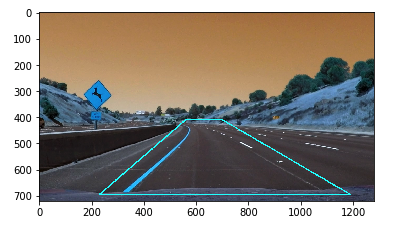
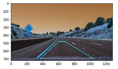
return combined_binary- Define the Outter and Inner Mask
mask = np.zeros_like(after_gradient_thresholding_imgs[0])
img_tmp = np.copy(original_images[0])
height = 720
length = 1280
left_down = (230, height - 25)
left_top = (560, 410)
right_top = (700, 410)
right_down = (length - 90, height - 25)
trapezoid_outter = np.array([[left_down, left_top, right_top, right_down]])
cv2.fillPoly(mask, trapezoid_outter, 255)
result = cv2.polylines(img_tmp, [trapezoid_outter], True, (0,255,255), 3)
plt.imshow(result)
mask = np.zeros_like(after_gradient_thresholding_imgs[0])
img_tmp = np.copy(original_images[0])
height = 720
length = 1280
left_down = (370, height - 25)
left_top = (600, 480)
right_top = (680, 480)
right_down = (length - 240, height - 25)
trapezoid_inner = np.array([[left_down, left_top, right_top, right_down]])
cv2.fillPoly(mask, trapezoid_inner, 255)
result = cv2.polylines(img_tmp, [trapezoid_inner], True, (0,255,255), 3)
plt.imshow(result)- Combine Color and Gradient Thresholding with Mask
def thresholding_with_mask(img, trapezoid_out, trapezoid_in):
    color_thresh = color_thresholding(img)
    gradient_thresh = gradient_threshold(img)

    combined_binary = np.zeros_like(gradient_thresh)
    combined_binary[(color_thresh == 1) | (gradient_thresh == 1)] = 1

    after_mask = region_of_interest(combined_binary, trapezoid_out, trapezoid_in)
    return after_mask
Here's the final output for this step.
3. Describe how (and identify where in your code) you performed a perspective transform and provide an example of a transformed image.
The code for my perspective transform includes a function called warp(), which appears in section 5 Perspective Transformation. The warp() function takes as inputs an image (img), as well as perspective transformation matrix M. I chose the hardcode the source and destination points in the following manner:
def calculate_M_Minv():
    height = 720
    length = 1280

    # Four source coordinates
    src = np.float32([
        [210, height],
        [595, 450],
        [690, 450],
        [1110, height]
    ])

    # Four desired coordinates
    dst = np.float32([
        [200, height],
        [200, 0],
        [1000, 0],
        [1000, height]
    ])

    # Compute the perspective transform matrix, M
    M = cv2.getPerspectiveTransform(src, dst)
    Minv = cv2.getPerspectiveTransform(dst, src)
    return M, Minv
This resulted in the following source and destination points:
| Source | Destination |
|---|---|
| 210, 720 | 200, 720 |
| 595, 450 | 200, 0 |
| 690, 450 | 1000, 0 |
| 1110, 720 | 1000, 0 |
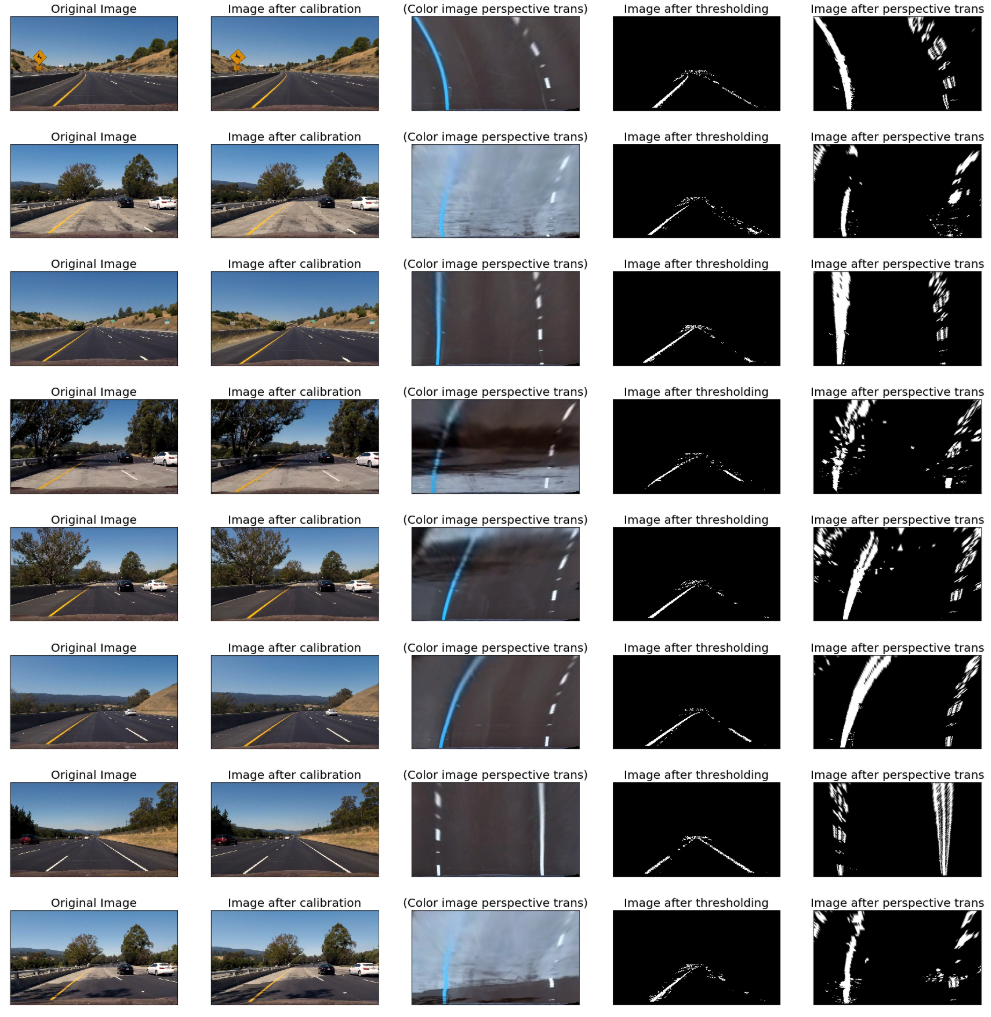
I verified that my perspective transform was working as expected by drawing the src and dst points onto a test image and its warped counterpart to verify that the lines appear parallel in the warped image.
4. Describe how (and identify where in your code) you identified lane-line pixels and fit their positions with a polynomial?
This part of code is in section 6 Finding the Lines.
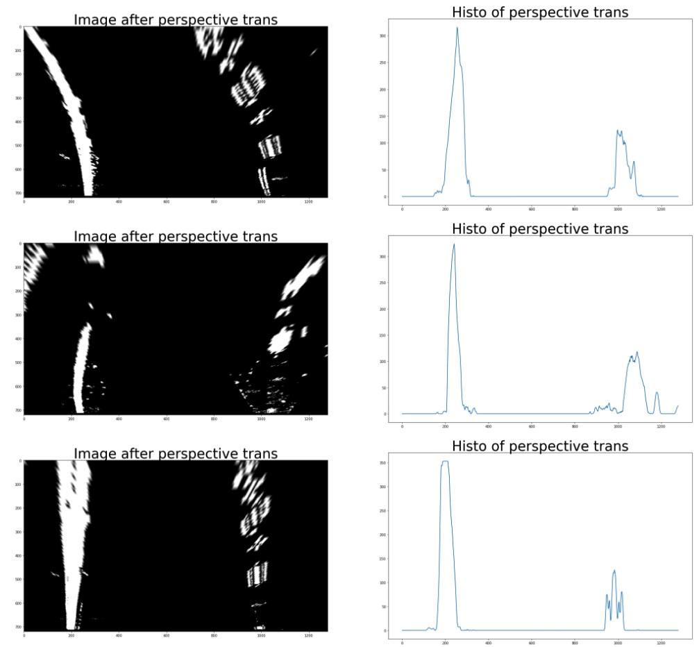
First I using histogram to analysis which part of binary wrapped image may contains the lane line. The peak in the plot shows the most potential position of starting point of lane line on the image. Here is the histogram I found:
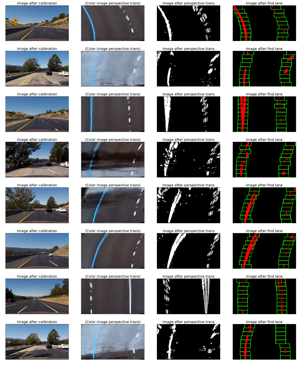
After that, I using a Sliding Window technique to find the pixels belong to the left line and right line. Here is the sliding window for some test images:
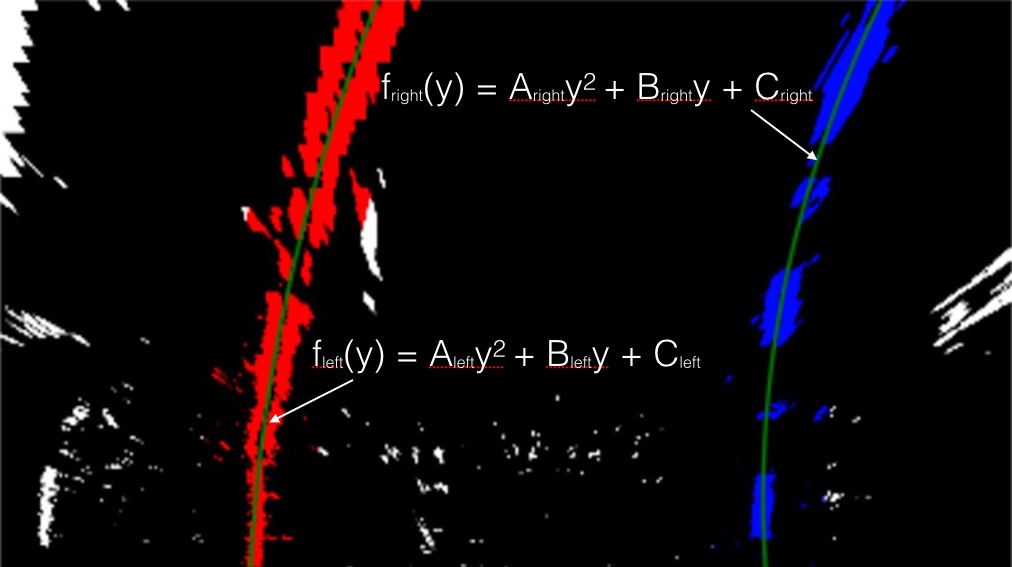
And Finally, I fit my lane lines with a 2nd order polynomial kinda like this:
5. Describe how (and identify where in your code) you calculated the radius of curvature of the lane and the position of the vehicle with respect to center.
The code is in section 7 Calculate radius and offset.
def measure_curvature_real(leftx, lefty, rightx, righty):
    '''
    Calculates the curvature of polynomial functions in meters.
    '''
    # Define conversions in x and y from pixels space to meters
    ym_per_pix = 30/720 # meters per pixel in y dimension
    xm_per_pix = 3.7/700 # meters per pixel in x dimension

    left_fit_cr = np.polyfit(lefty * ym_per_pix, leftx * xm_per_pix, 2)
    right_fit_cr = np.polyfit(righty * ym_per_pix, rightx * xm_per_pix, 2)

    # Define y-value where we want radius of curvature
    # We'll choose the maximum y-value, corresponding to the bottom of the image
    y_eval = 720

    # Calculation of R_curve (radius of curvature)
    left_curverad = ((1 + (2 * left_fit_cr[0] * y_eval * ym_per_pix + left_fit_cr[1])**2)**1.5) / np.absolute(2 * left_fit_cr[0])
    right_curverad = ((1 + (2 * right_fit_cr[0] * y_eval * ym_per_pix + right_fit_cr[1])**2)**1.5) / np.absolute(2 * right_fit_cr[0])
    radius = (left_curverad + right_curverad) / 2
    offset = (640 - (leftx[-1] + rightx[-1]) / 2) * xm_per_pix

    return radius, offset
6. Provide an example image of your result plotted back down onto the road such that the lane area is identified clearly.
I implemented this step in section 6.3 Draw lane line and unwarp back to original perspective and 8 The Final Pipeline.
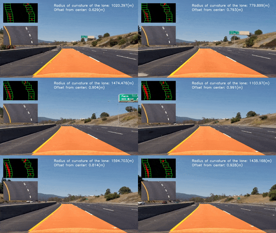
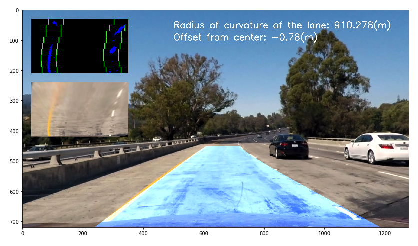
In addition, I also added two subplot into the final result
- The lane line in the bird view.
- The Sliding Window with Binary Wrapped Line. These two subplot can illustrate the overall pipeline more clear.
Here is an example of my result on a test image:
1. Provide a link to your final video output. Your pipeline should perform reasonably well on the entire project video (wobbly lines are ok but no catastrophic failures that would cause the car to drive off the road!).
Here's a link to my video result
Also in youtube: https://youtu.be/NfRKwuZLWsI
1. Briefly discuss any problems / issues you faced in your implementation of this project. Where will your pipeline likely fail? What could you do to make it more robust?
First I want the thresholding step is very tricky. I found this part is very important to the rest part of the project. If the binary wrapped images cannot properly illustrate the lane line, there is noway of to use fit them into the right polynomial lanes. I did a lot of combination experiment around the color space selection, and finally picked a robust one.
Secondly, when finding the lane line, I am using sliding window technique, which will examine the whole image frame by frame. As the lecture said, using the search from prior can reduce the unnecessary searching computation. And also convolution way also can be used to improve this part.
As for the drawback of the current pipeline, the change of the lightweight, different weather condition, and the lack of clear laneline, vehicle in front of laneline, different position of camera on my car, all of them will break the pipeline. So there definitely a long way to go to achieve a general purpose advanced lane line detection solution. But I am very passion on it, and will keep study.
My OS: Ubuntu 16.04
- Download https://github.com/imageio/imageio-binaries/raw/master/ffmpeg/ffmpeg-linux64-v3.3.1
- Save it to filename: /home/yourname/.imageio/ffmpeg/ffmpeg-linux64-v3.3.1
- run
pip install requests
