The goals / steps of this project are the following:
- Perform a Histogram of Oriented Gradients (HOG) feature extraction on a labeled training set of images and train a classifier Linear SVM classifier
- Optionally, you can also apply a color transform and append binned color features, as well as histograms of color, to your HOG feature vector.
- Note: for those first two steps don't forget to normalize your features and randomize a selection for training and testing.
- Implement a sliding-window technique and use your trained classifier to search for vehicles in images.
- Run your pipeline on a video stream (start with the test_video.mp4 and later implement on full project_video.mp4) and create a heat map of recurring detections frame by frame to reject outliers and follow detected vehicles.
- Estimate a bounding box for vehicles detected.
1. Explain how (and identify where in your code) you extracted HOG features from the training images.
The code for this step is contained in the section 5 Extract HOG Features. The code is as bellow:
def get_hog_features(img,
                     orient = 8,
                     pix_per_cell = 8,
                     cell_per_block = 2,
                     vis = True,
                     feature_vec = True,
                     trans_sqrt = True):

    """
    Function accepts params and returns HOG features (optionally flattened) and an optional matrix for
    visualization. Features will always be the first return (flattened if feature_vector= True).
    A visualization matrix will be the second return if visualize = True.
    """

    return_list = hog(img,
                      orientations = orient,
                      pixels_per_cell = (pix_per_cell, pix_per_cell),
                      cells_per_block = (cell_per_block, cell_per_block),
                      block_norm = 'L2-Hys',
                      transform_sqrt = trans_sqrt,
                      visualize = vis,
                      feature_vector = feature_vec)

    if vis:
        hog_features = return_list[0]
        hog_image = return_list[1]
        return hog_features, hog_image
    else:
        return return_list
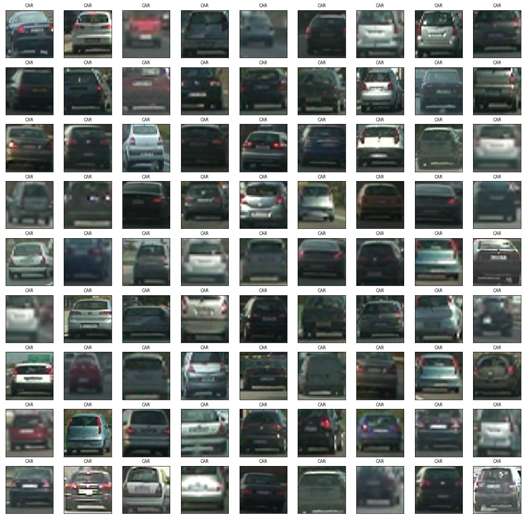
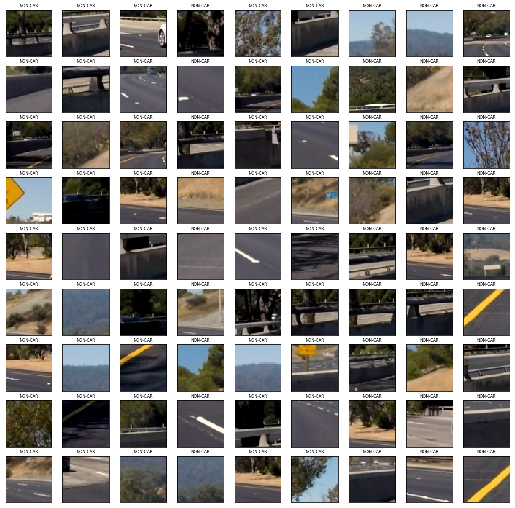
Let's first take a look of the training data. Training data contains two categories, one for car, the other is non-car. Here is some sample images:
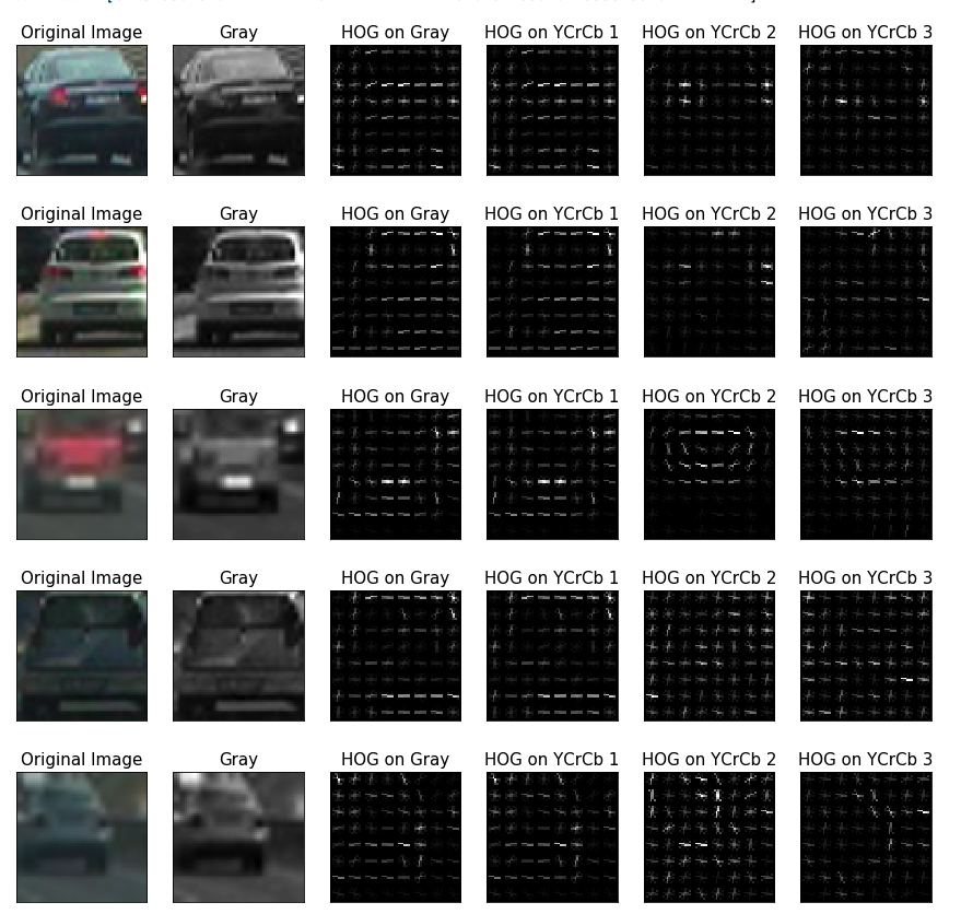
I then explored different color spaces and different skimage.hog() parameters (orientations, pixels_per_cell, and cells_per_block). I grabbed random images from each of the two classes and displayed them to get a feel for what the skimage.hog() output looks like.
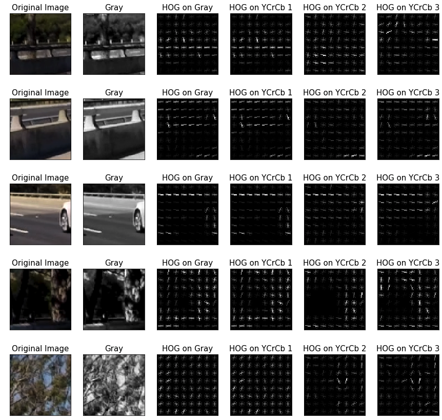
Here is an example using the YCrCb colour space and HOG parameters of orientations=8, pixels_per_cell=(8, 8) and cells_per_block=(2, 2):
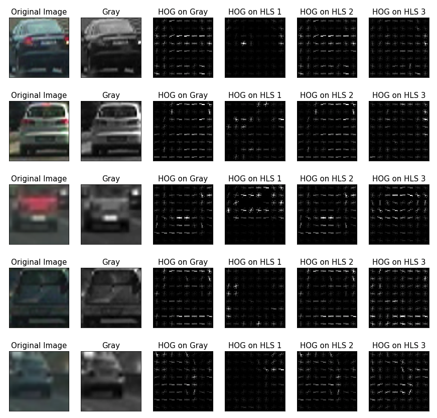
And there is a example of another colour space (HLS) for same HOG parameters:
We can see there are some different in visualisation. But I can tell, colour space different didn't impact much of the model quality. This can be proved by the bellow classifier experiments.
Let's see an example of non car HOG visualisation:
I tried various combinations of parameters and finally using this combination:
orient = 8,
pix_per_cell = 8,
cell_per_block = 2,
block_norm = 'L2-Hys',
transform_sqrt = True
3. Describe how (and identify where in your code) you trained a classifier using your selected HOG features (and color features if you used them).
I trained a linear SVM using HOG plus Spatial Features and Color Histogram Features. The whole feature combination as follow:
def extract_features(imgs,
                     cspace = 'YCrCb',
                     orient = 9,
                     pix_per_cell = 16,
                     cell_per_block = 1,
                     hog_channel = 'ALL',
                     spatial_feat = True,
                     hist_feat = True):

    # Create a list to append feature vectors to
    features = []

    # Iterate through the list of images
    for file in imgs:
        single_feature = []
        # Read in each one by one
        image = mpimg.imread(file)
        # apply color conversion if other than 'RGB'
        if cspace != 'RGB':
            if cspace == 'HSV':
                feature_image = cv2.cvtColor(image, cv2.COLOR_RGB2HSV)
            elif cspace == 'LUV':
                feature_image = cv2.cvtColor(image, cv2.COLOR_RGB2LUV)
            elif cspace == 'HLS':
                feature_image = cv2.cvtColor(image, cv2.COLOR_RGB2HLS)
            elif cspace == 'YUV':
                feature_image = cv2.cvtColor(image, cv2.COLOR_RGB2YUV)
            elif cspace == 'YCrCb':
                feature_image = cv2.cvtColor(image, cv2.COLOR_RGB2YCrCb)
        else: feature_image = np.copy(image)

        if spatial_feat == True:
            spatial_features = bin_spatial(feature_image, size = (16,16))
            single_feature.append(spatial_features)
        if hist_feat == True:

            hist_features = color_hist(feature_image, nbins = 32)
            single_feature.append(hist_features)

        # Call get_hog_features() with vis=False, feature_vec=True
        if hog_channel == 'ALL':
            hog_features = []
            for channel in range(feature_image.shape[2]):
                hog_features.append(get_hog_features(feature_image[:, :, channel],
                                    orient,
                                    pix_per_cell,
                                    cell_per_block,
                                    vis = False,
                                    feature_vec = True))
            hog_features = np.ravel(hog_features)
        else:
            hog_features = get_hog_features(feature_image[:, :, hog_channel],
                                            orient,
                                            pix_per_cell,
                                            cell_per_block,
                                            vis = False,
                                            feature_vec = True)

        # Append the new feature vector to the features list
        single_feature.append(hog_features)

        features.append(np.concatenate(single_feature))

    # Return list of feature vectors
    return features
This is the pipe line I used to train the classifier:
colorspace = 'YCrCb' # Can be RGB, HSV, LUV, HLS, YUV, YCrCb
# orient = 9
# pix_per_cell = 16
# cell_per_block = 1
orient = 8
pix_per_cell = 8
cell_per_block = 2
hog_channel = "ALL" # Can be 0, 1, 2, or "ALL"

t = time.time()

car_features = extract_features(car_paths,
                                cspace = colorspace,
                                orient = orient,
                                pix_per_cell = pix_per_cell,
                                cell_per_block = cell_per_block,
                                hog_channel = hog_channel)

notcar_features = extract_features(non_car_paths,
                                   cspace = colorspace,
                                   orient = orient,
                                   pix_per_cell = pix_per_cell,
                                   cell_per_block = cell_per_block,
                                   hog_channel = hog_channel)

t2 = time.time()

print(round(t2 - t, 2), 'Seconds to extract HOG features...')

# Create an array stack of feature vectors
X = np.vstack((car_features, notcar_features)).astype(np.float64)

# Define the labels vector
y = np.hstack((np.ones(len(car_features)),
               np.zeros(len(notcar_features))
             ))

# Split up data into randomized training and test sets
rand_state = np.random.randint(0, 100)

X_train, X_test, y_train, y_test = train_test_split(X,
                                                    y,
                                                    test_size = 0.2,
                                                    random_state = rand_state)

# Fit a per-column scaler
X_scaler = StandardScaler().fit(X_train)

# Apply the scaler to X
X_train = X_scaler.transform(X_train)
X_test = X_scaler.transform(X_test)

print('Using:', orient, 'orientations',
                pix_per_cell, 'pixels per cell and',
                cell_per_block,'cells per block')

print('Feature vector length:', len(X_train[0]))

# Use a linear SVC
svc = LinearSVC()

# Check the training time for the SVC
t = time.time()
svc.fit(X_train, y_train)
t2 = time.time()
print(round(t2 - t, 2), 'Seconds to train SVC...')

# Check the score of the SVC
print('Test Accuracy of SVC = ', round(svc.score(X_test, y_test), 4))

# Check the prediction time for a single sample
t = time.time()
n_predict = 10
print('My SVC predicts: ', svc.predict(X_test[0:n_predict]))
print('For these',n_predict, 'labels: ', y_test[0:n_predict])
t2 = time.time()
print(round(t2 - t, 5), 'Seconds to predict', n_predict,'labels with SVC')
I made several experiments, here is the outcome:
- I found multi features combination provide better model performance then single HOG feature model. When I only use HOG as feature, I can only get
0.96Test Accuracy. After I add Spatial and Color Histogram features, although the whole feature length expand to 5568 from 1766 for a single image, the final Test Accuracy increase to0.99 - And I also try different color space for HOG. The result shows there are not very much difference.
- Using
YCrCb, Test Accuracy of Classifier is0.9882 - Using
HLS, Test Accuracy of Classifier is0.9896 - Ref section
7 Training the Classifier with different hyper parameters
- Using
1. Describe how (and identify where in your code) you implemented a sliding window search. How did you decide what scales to search and how much to overlap windows?
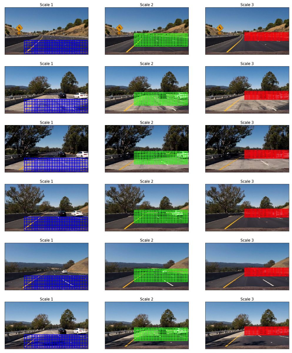
I decided to find the car using multi scale sliding window mechanism, Let's first take a look of my search schema:
I am using 3 different window, the more close to the central, the smaller the window is, and also the more overlap of the window is. Here is the code to define the 3 window I am using:
def multi_scale_window(image):
    x_limits = [[300, None],
                [450, None],
                [600, None]]

    y_limits = [[540, None],
                [400, 600],
                [380, 520]]

    window_size = [(128, 128),
                   (96, 96),
                   (72, 72)]

    overlap_ratio = [(0.7, 0.7),
                     (0.75, 0.75),
                     (0.8, 0.8)]

    all_windows = []

    for x_limit, y_limit, size, overlap in zip (x_limits,
                                                y_limits,
                                                window_size,
                                                overlap_ratio):
        windows = slide_window(
            image,
            x_start_stop = x_limit,
            y_start_stop = y_limit,
            xy_window = size,
            xy_overlap = overlap
        )
        all_windows.extend(windows)

    return all_windows
2. Show some examples of test images to demonstrate how your pipeline is working. What did you do to optimize the performance of your classifier?
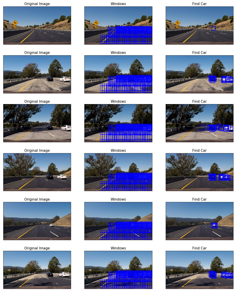
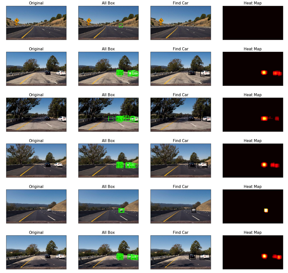
Ultimately I searched on three scales using YCrCb 3-channel HOG features plus spatially binned color and histograms of color in the feature vector, which provided a nice result. Here are some example images:
I have try to use the HOG Sub-Sampling Windows Search mechanism to optimize the performance. It indeed can accelerate the performance a lot, like around 8x time. But I finally didn't use this technique in my final pipeline. One reason is I found my multi scale window schema can generate better result than de Sub-Sampling Windows Search mechanism, I believe after fine tune the Sub-Sampling code, it can produce same performance as my multi scale window. Another reason I didn't proceed the fine tune of Sub-Sampling is I want to try YOLOv3 later, which can also produce a fast and more accurate result.
1. Provide a link to your final video output. Your pipeline should perform reasonably well on the entire project video (somewhat wobbly or unstable bounding boxes are ok as long as you are identifying the vehicles most of the time with minimal false positives.)
Here's the link to my video result in Youtube
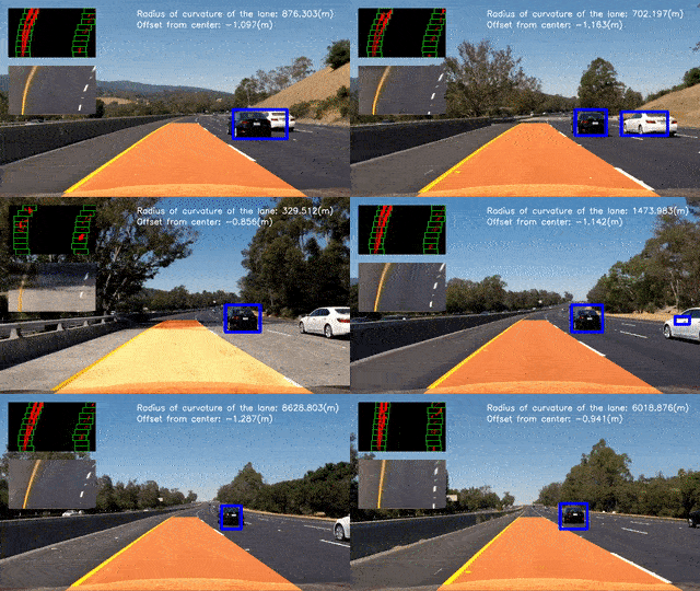
I also integrate the vehicle detection with the advanced lane line detection. Here's the link to my the integration video in Youtube
2. Describe how (and identify where in your code) you implemented some kind of filter for false positives and some method for combining overlapping bounding boxes.
I recorded the positions of positive detections in each frame of the video. From the positive detections I created a heatmap and then thresholded that map to identify vehicle positions. I then used scipy.ndimage.measurements.label() to identify individual blobs in the heatmap. I then assumed each blob corresponded to a vehicle. I constructed bounding boxes to cover the area of each blob detected.
Here's an example result showing the heatmap from a series of frames of video, the result of scipy.ndimage.measurements.label() and the bounding boxes then overlaid on the last frame of video:
1. Briefly discuss any problems / issues you faced in your implementation of this project. Where will your pipeline likely fail? What could you do to make it more robust?
Here is my thoughts:
- As I memtioned above, HOG sub-sampling would be one of field need further fine tune, which can accelerate the searching performance.
- And track the bounding boxes in last n frames, and using the average of these bounding boxes can make the labelling more stable, not like current joggling bounding box.
- Using more robust classifier, such mask-rcnn / faster-rcnn / yolov3 to replace current SVM classifier.
- I suspect the weather condition, light condition, different type and color of car/vehicle(eg, truck) may fail the pipeline.
Yang
