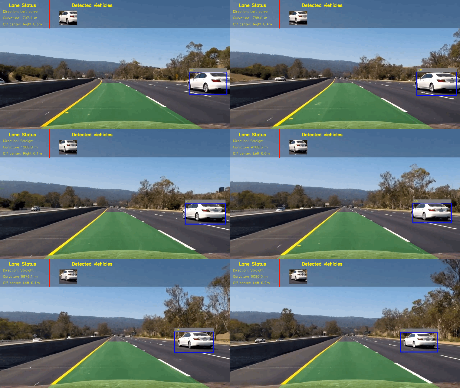
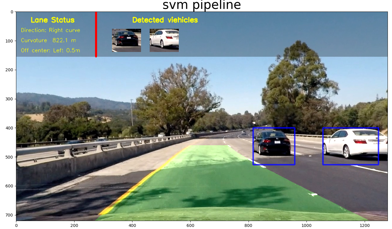
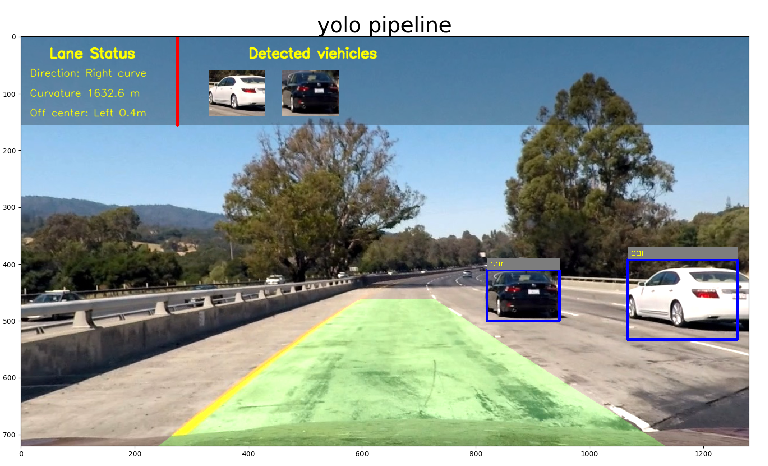
(1) Highway Drive (with Lane Departure Warning) (Click to see the full video)
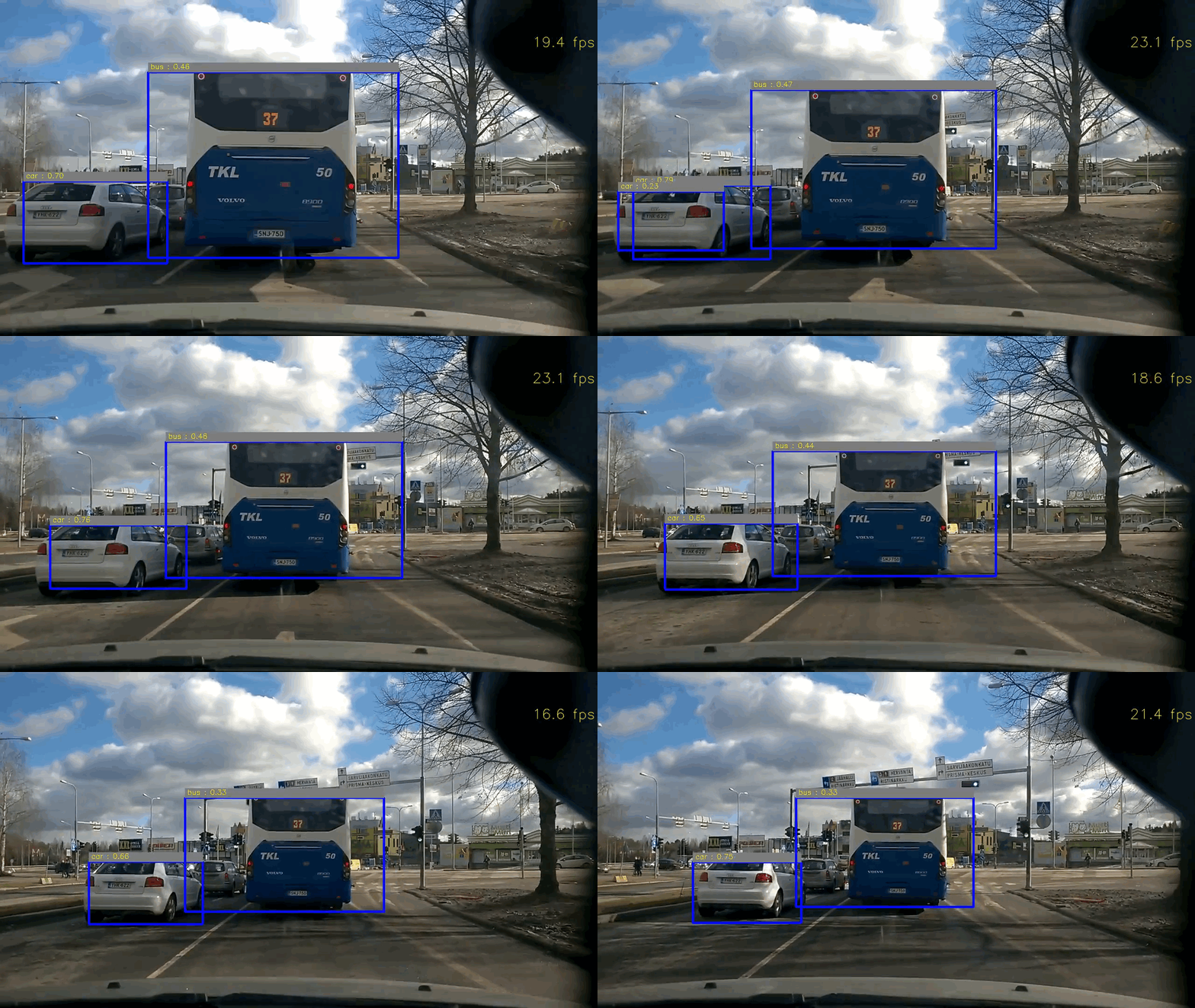
(2) City Drive (Vehicle Detection only) (Click to see the full video)
- main.py is the main code for demos
- svm_pipeline.py is the car detection pipeline with SVM
- yolo_pipeline.py is the car detection pipeline with a deep net YOLO (You Only Look Once)
- visualization.py is the function for adding visalization
Others are the same as in the repository of Lane Departure Warning System:
- calibration.py contains the script to calibrate camera and save the calibration results
- lane.py contains the lane class
- examples folder contains the sample images and videos
Anaconda is used for managing my dependencies.
- OpenCV3, Python3.5, tensorflow, CUDA8
- OS: Ubuntu 16.04
(1) Download weights for YOLO
You can download the weight from here and save it to the weights folder.
(2) If you want to run the demo, you can simply run:
python main.py-
0.1.1
- Fix two minor bugs and update the documents
- Date 18 April 2017
-
0.1.0
- The first proper release
- Date 31 March 2017
svm_pipeline.py contains the code for the svm pipeline.
Steps:
- Perform a Histogram of Oriented Gradients (HOG) feature extraction on a labeled training set of images and train a classifier Linear SVM classifier
- A color transform is applied to the image and append binned color features, as well as histograms of color, to HOG feature vector.
- Normalize your features and randomize a selection for training and testing.
- Implement a sliding-window technique and use SVM classifier to search for vehicles in images.
- Run pipeline on a video stream and create a heat map of recurring detections frame by frame to reject outliers and follow detected vehicles.
- Estimate a bounding box for detected vehicles.
The code for this step is contained in the function named extract_features and codes from line 464 to 552 in svm_pipeline.py.
If the SVM classifier exist, load it directly.
Otherwise, I started by reading in all the vehicle and non-vehicle images, around 8000 images in each category. These datasets are comprised of
images taken from the GTI vehicle image database and
KITTI vision benchmark suite.
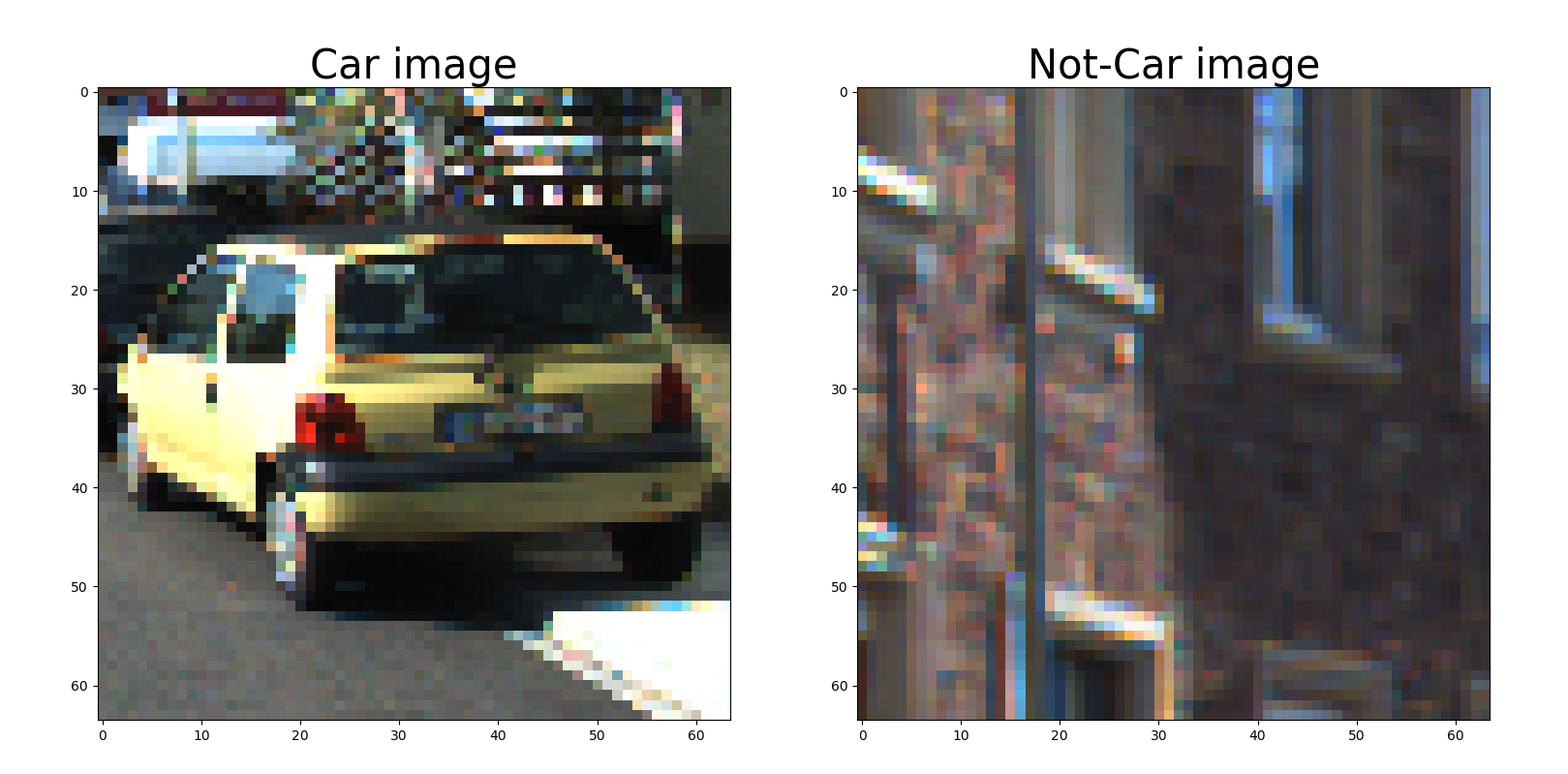
Here is an example of one of each of the vehicle and non-vehicle classes:
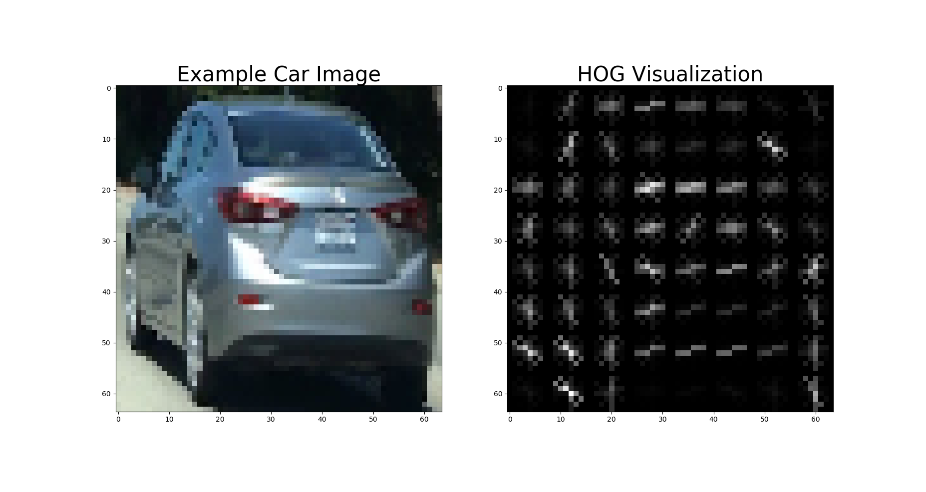
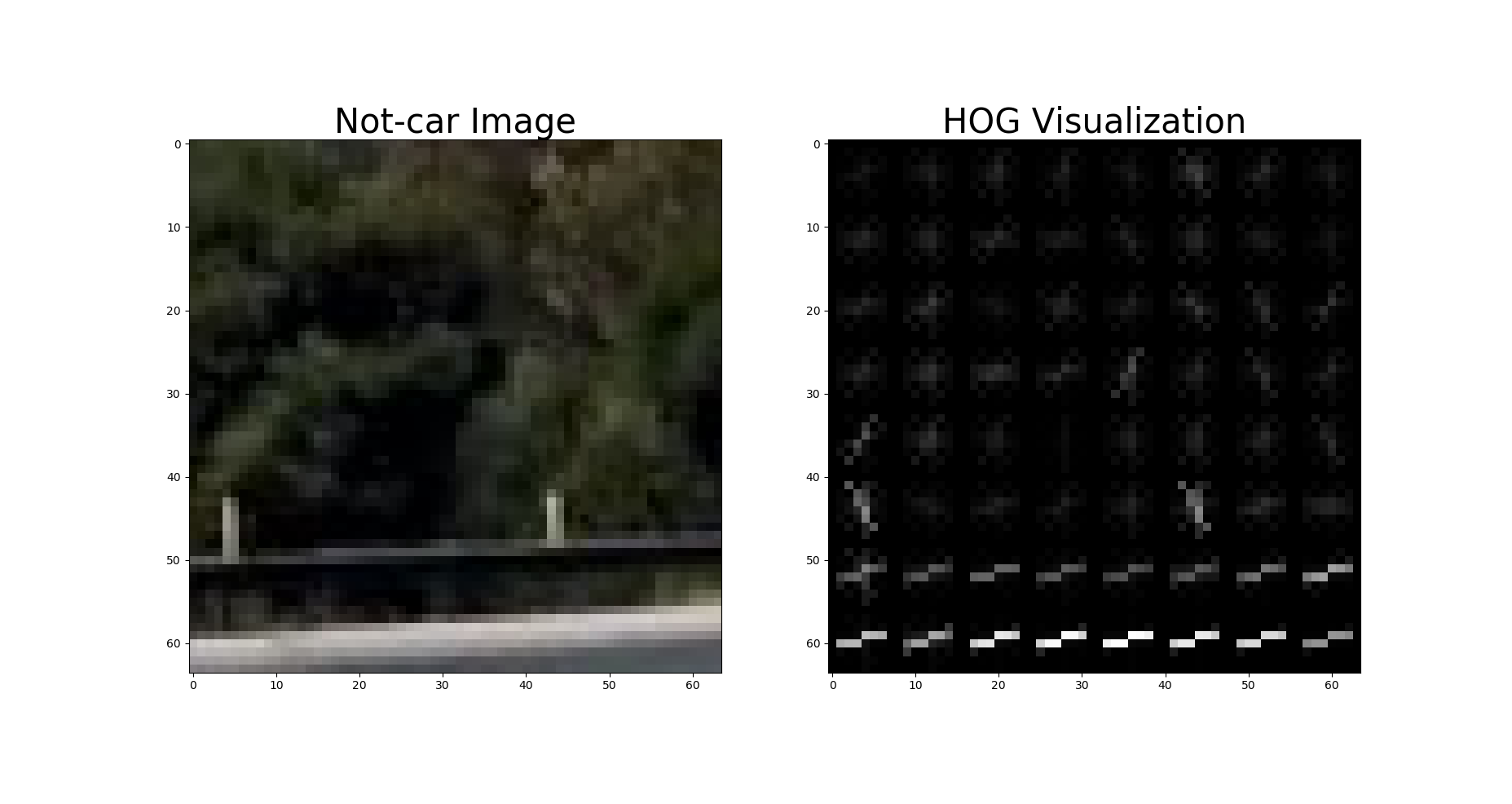
I then explored different color spaces and different skimage.hog() parameters (orientations, pixels_per_cell, and cells_per_block). I grabbed random images from each of the two classes and displayed them to get a feel for what the skimage.hog() output looks like.
Here is an example using the RGB color space and HOG parameters of orientations=9, pixels_per_cell=(8, 8) and cells_per_block=(2, 2):
To optimize the HoG extraction, I extract the HoG feature for the entire image only once. Then the entire HoG image
is saved for further processing. (see line 319 to 321 in svm_pipeline.py)
I tried various combinations of parameters and choose the final combination as follows
(see line 16-27 in svm_pipeline.py):
YCrCbcolor space- orient = 9 # HOG orientations
- pix_per_cell = 8 # HOG pixels per cell
- cell_per_block = 2 # HOG cells per block, which can handel e.g. shadows
- hog_channel = "ALL" # Can be 0, 1, 2, or "ALL"
- spatial_size = (32, 32) # Spatial binning dimensions
- hist_bins = 32 # Number of histogram bins
- spatial_feat = True # Spatial features on or off
- hist_feat = True # Histogram features on or off
- hog_feat = True # HOG features on or off
All the features are normalized by line 511 to 513 in svm_pipeline.py, which is a critical step. Otherwise, classifier
may have some bias toward to the features with higher weights.
I randomly select 20% of images for testing and others for training, and a linear SVM is used as classifier (see line
520 to 531 in svm_pipeline.py)
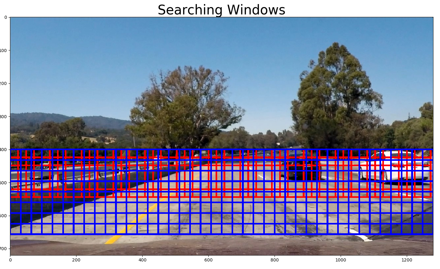
For this SVM-based approach, I use two scales of the search window (64x64 and 128x128, see line 41) and search only between
[400, 656] in y axis (see line 32 in svm_pipeline.py). I choose 75% overlap for the search windows in each scale (see
line 314 in svm_pipeline.py).
For every window, the SVM classifier is used to predict whether it contains a car nor not. If yes, save this window (see
line 361 to 366 in svm_pipeline.py). In the end, a list of windows contains detected cars are obtianed.
After obtained a list of windows which may contain cars, a function named generate_heatmap (in line 565 in
svm_pipeline.py) is used to generate a heatmap. Then a threshold is used to filter out the false positives.
For image, we could directly use the result from the filtered heatmap to create a bounding box of the detected vehicle.
For video, we could further utilize neighbouring frames to filter out the false positives, as well as to smooth the position of bounding box.
- Accumulate the heatmap for N previous frame.
- Apply weights to N previous frames: smaller weights for older frames (line 398 to 399 in
svm_pipeline.py). - I then apply threshold and use
scipy.ndimage.measurements.label()to identify individual blobs in the heatmap. - I then assume each blob corresponded to a vehicle and constructe bounding boxes to cover the area of each blob detected.
yolo_pipeline.py contains the code for the yolo pipeline.
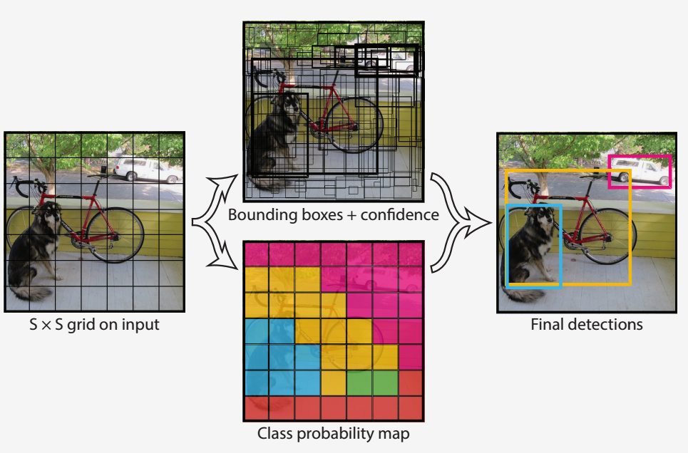
YOLO is an object detection pipeline baesd on Neural Network. Contrast to prior work on object detection with classifiers to perform detection, YOLO frame object detection as a regression problem to spatially separated bounding boxes and associated class probabilities. A single neural network predicts bounding boxes and class probabilities directly from full images in one evaluation. Since the whole detection pipeline is a single network, it can be optimized end-to-end directly on detection performance.
Steps to use the YOLO for detection:
- resize input image to 448x448
- run a single convolutional network on the image
- threshold the resulting detections by the model’s confidence
yolo_pipeline.py is modified and integrated based on this tensorflow implementation of YOLO.
Since the "car" is known to YOLO, I use the precomputed weights directly and apply to the entire input frame.
For the SVM based approach, the accuray is good, but the speed (2 fps) is an problem due to the fact of sliding window approach is time consuming! We could use image downsampling, multi-threads, or GPU processing to improve the speed. But, there are probably a lot engineering work need to be done to make it running real-time. Also, in this application, I limit the vertical searching range to control the number of searching windows, as well as avoid some false positives (e.g. cars on the tree).
For YOLO based approach, it achieves real-time and the accuracy are quite satisfactory. Only in some cases, it may failure to detect the small car thumbnail in distance. My intuition is that the original input image is in resolution of 1280x720, and it needs to be downscaled to 448x448, so the car in distance will be tiny and probably quite distorted in the downscaled image (448x448). In order to correctly identify the car in distance, we might need to either crop the image instead of directly downscaling it, or retrain the network.
