The goal of this project is to develop a pipeline to process a video stream from a forward-facing camera mounted on the front of a car, and output an annotated video which identifies:
- The positions of the lane lines
- The location of the vehicle relative to the center of the lane
- The radius of curvature of the road
The pipeline created for this project processes images in the following steps:
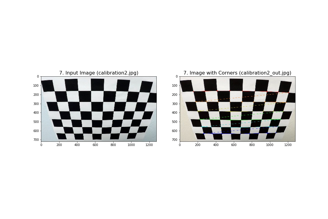
- Step 1: Compute the camera calibration matrix and distortion coefficients given a set of chessboard images.
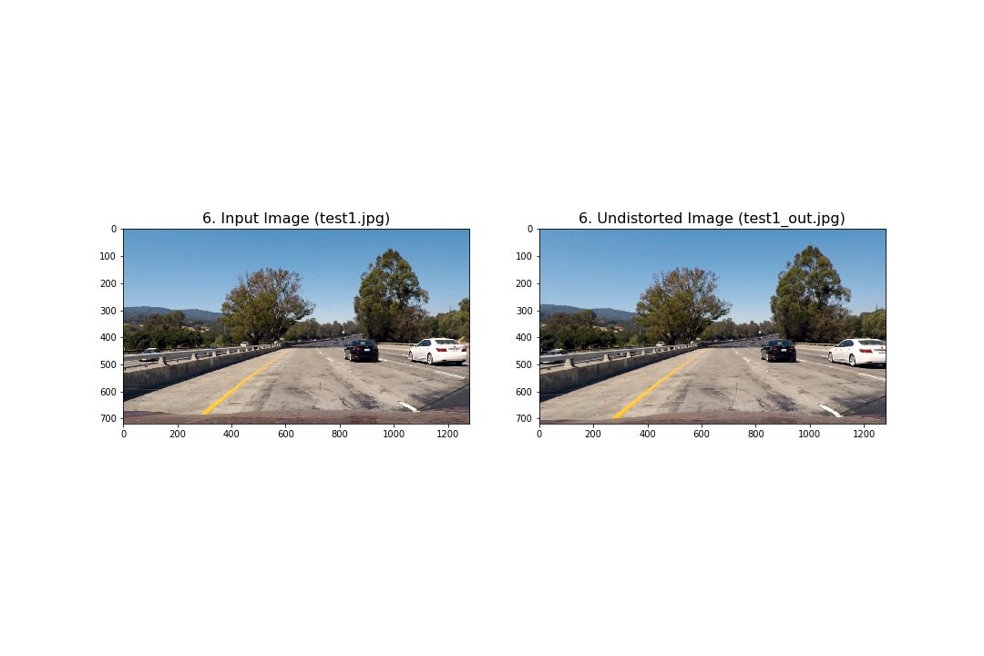
- Step 2: Apply a distortion correction to raw images.
- Step 3: Apply a perspective transform to rectify binary image ("birds-eye view").
- Step 4: Use color transforms, gradients, etc., to create a thresholded binary image.
- Step 5: Detect lane pixels and fit to find the lane boundary.
- Step 6: Determine the curvature of the lane and vehicle position with respect to center.
- Step 7: Warp the detected lane boundaries back onto the original image.
- Step 8: Output visual display of the lane boundaries and numerical estimation of lane curvature and vehicle position.
In this step, I used the OpenCV functions findChessboardCorners and drawChessboardCorners to identify the locations of corners on a series of pictures of a chessboard taken from different angles.
Next, the locations of the chessboard corners were used as input to the OpenCV function calibrateCamera to compute the camera calibration matrix and distortion coefficients.
Finally, the camera calibration matrix and distortion coefficients were used with the OpenCV function undistort to remove distortion from highway driving images.
Notice that if you compare the two images, especially around the edges, there are obvious differences between the original and undistorted image, indicating that distortion has been removed from the original image.
The goal of this step is to transform the undistorted image to a "birds eye view" of the road which focuses only on the lane lines and displays them in such a way that they appear to be relatively parallel to eachother (as opposed to the converging lines you would normally see). To achieve the perspective transformation I first applied the OpenCV functions getPerspectiveTransform and warpPerspective which take a matrix of four source points on the undistorted image and remaps them to four destination points on the warped image. The source and destination points were selected manually by visualizing the locations of the lane lines on a series of test images.
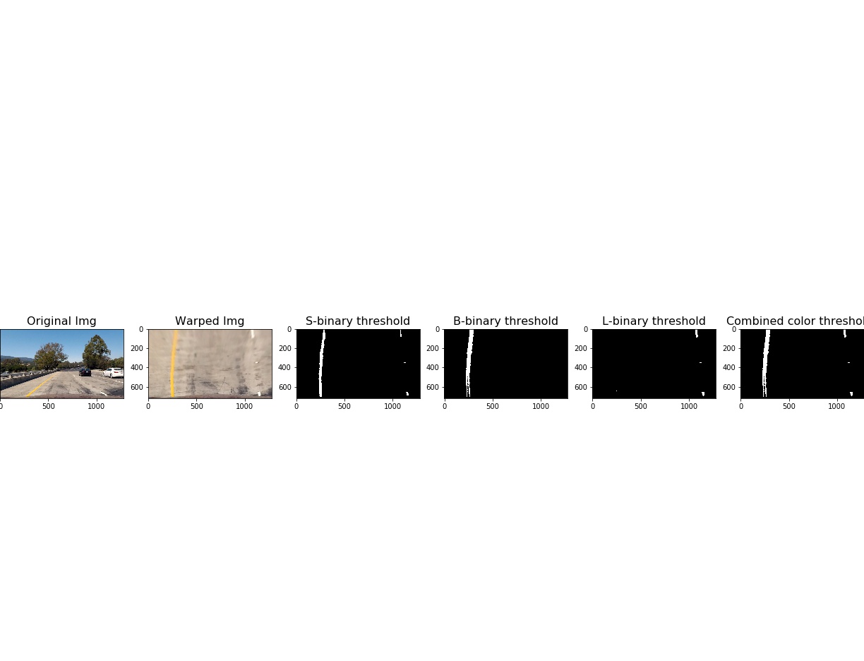
In this step I attempted to convert the warped image to different color spaces and create binary thresholded images which highlight only the lane lines and ignore everything else. I found that the following color channels and thresholds did a good job of identifying the lane lines in the provided test images:
- The S Channel from the HLS color space, with a min threshold of 180 and a max threshold of 255, did a fairly good job of identifying both the white and yellow lane lines, but did not pick up 100% of the pixels in either one, and had a tendency to get distracted by shadows on the road.
- The L Channel from the LUV color space, with a min threshold of 225 and a max threshold of 255, did an almost perfect job of picking up the white lane lines, but completely ignored the yellow lines.
- The B channel from the Lab color space, with a min threshold of 155 and an upper threshold of 200, did a better job than the S channel in identifying the yellow lines, but completely ignored the white lines.
I chose to create a combined binary threshold based on the three above mentioned binary thresholds, to create one combination thresholded image which does a great job of highlighting almost all of the white and yellow lane lines.
At this point I was able to use the combined binary image to isolate only the pixels belonging to lane lines. The next step was to fit a polynomial to each lane line, which was done by:
- Identifying peaks in a histogram of the image to determine location of lane lines.
- Identifying all non zero pixels around histogram peaks using the numpy function
np.nonzero(). - Fitting a polynomial to each lane using the numpy function
np.polyfit().
After fitting the polynomials I was able to calculate the position of the vehicle with respect to center with the following calculations:
- Calculated the average of the x intercepts from each of the two polynomials ;
- Calculated the distance from center by taking the absolute value of the vehicle position minus the halfway point along the horizontal axis;
- If the horizontal position of the car was greater than
image_width/2than the car was considered to be left of center, otherwise right of center. - Finally, the distance from center was converted from pixels to meters by multiplying the number of pixels by
3.7/700.
Next I used the following code to calculate the radius of curvature for each lane line in meters:
xm_per_pix = 3.7/700 # meteres/pixel in x dimension
ym_per_pix = 30.0/720 # meters/pixel in y dimension

left_lane_fit_curvature = np.polyfit(left_y*ym_per_pix, left_x*xm_per_pix, 2)
right_lane_fit_curvature = np.polyfit(right_y*ym_per_pix, right_x*xm_per_pix, 2)
radius_left_curve = ((1 + (2*left_lane_fit_curvature[0]*np.max(left_y) + left_lane_fit_curvature[1])**2)**1.5) \
/np.absolute(2*left_lane_fit_curvature[0])
radius_right_curve = ((1 + (2*right_lane_fit_curvature[0]*np.max(left_y) + right_lane_fit_curvature[1])**2)**1.5) \
/np.absolute(2*right_lane_fit_curvature[0])
In this step in processing the images was to plot the polynomials on to the warped image, fill the space between the polynomials to highlight the lane that the car is in, use another perspective trasformation to unwarp the image from birds eye back to its original perspective, and print the distance from center and radius of curvature on to the final annotated image.
- Step 8: Output visual display of the lane boundaries and numerical estimation of lane curvature and vehicle position.
The video pipeline developed in this project did a fairly robust job of detecting the lane lines in the test video provided for the project, which shows a road in basically ideal conditions, with fairly distinct lane lines, and on a clear day.
It also did a decent job with the challenge video, although it did lose the lane lines momentarily when there was heavy shadow over the road from an overpass.
However in the harder video is was really bad result
What I have learned from this project is that it is relatively easy to finetune a software pipeline to work well for consistent road and weather conditions, but what is challenging is finding a single combination which produces the same quality result in any condition. I have not yet tested the pipeline on additional video streams which could challenge the pipeline with varying lighting and weather conditions, road quality, faded lane lines, and different types of driving like lane shifts, passing, and exiting a highway. For further research I plan to record some additional video streams of my own driving in various conditions and continue to refine my pipeline to work in more varied environments.


