lindia

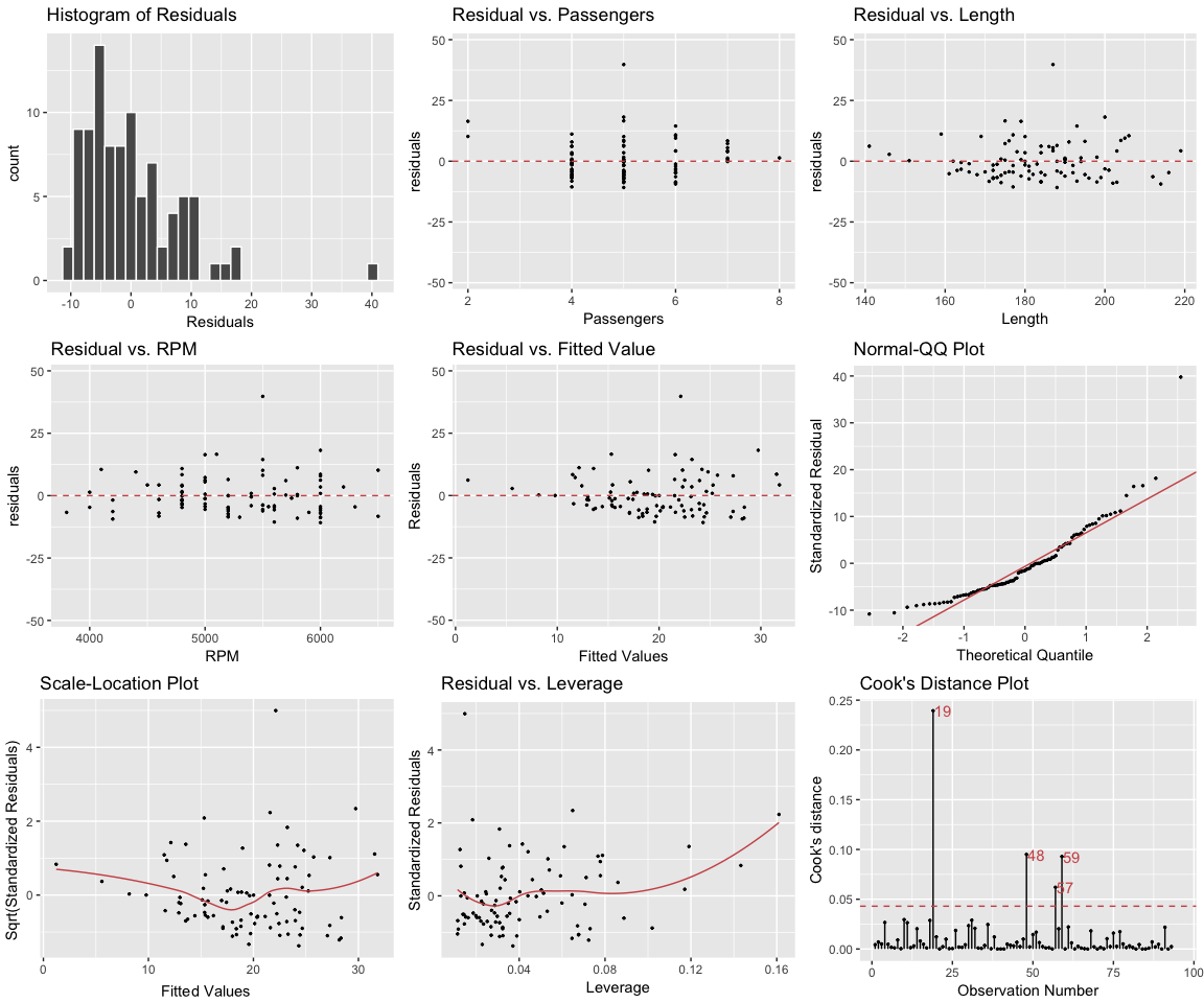
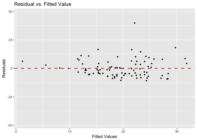
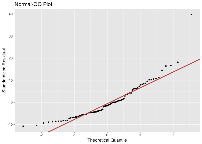
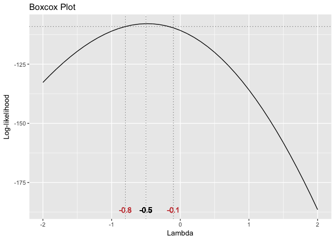
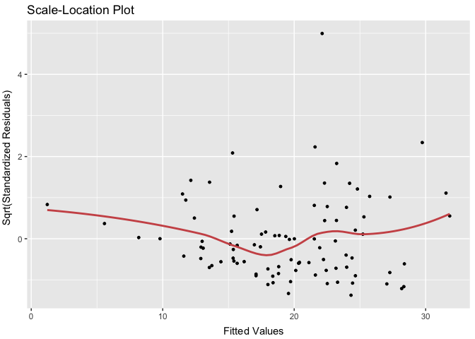
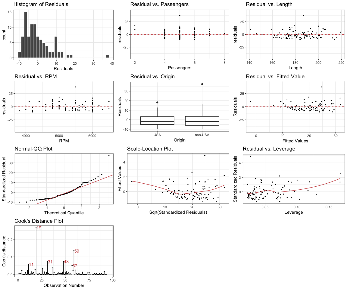
lindia is an extention to ggplot2 to provide streamlined plotting features of linear model diagnostic plots. The following demonstrates basic plotting features of lindia. All functions in lindia takes in an lm object (including lm() and glm()) and returns linear diagnostic plots in forms of ggplot objects. The following code demonstrates how you can create a simple linear model from Cars93 dataset, then use a call to lindia::gg_diagnose() to visualize overall features of the distribution.

# create linear model
cars_lm <- lm(Price ~ Passengers + Length + RPM, data = Cars93)

# visualize diagnostic plots with a call to lindia
gg_diagnose(cars_lm)

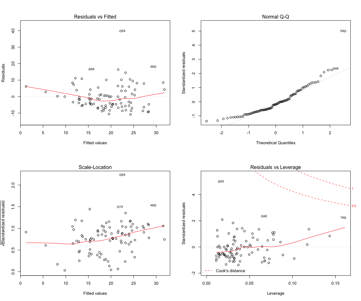
The functionality of lindia is an improvement of the features provided in base-R graphs. Using base-R, user can also create a series of diagnostic plots using the following line:

par(mfrow = c(2,2))
plot(cars_lm)

However, the output from a call to plot() lacks flexibility and comprehensiveness. For example, residual vs. predictor plots are not shown, and that users cannot easily maipulate graph type and aesthetics. In that sense, lindia is an extension to features offered in base-R.

Installation

From Github: devtools::install_github("yeukyul/lindia")

Overview

Followed are functions implemented in lindia:

gg_reshist(): Histogram of residuals
gg_resfitted(): Residual plot of residuals by fitted value
gg_resX(): All residual plots of all predictors by fitted value, layed out in a grid
gg_qqplot(): Normaility quantile-quantile plot (QQPlot) with qqline overlayed on top
gg_boxcox(): Boxcox graph with optimal transformation labeled on graph
gg_scalelocation(): Scale-location plot (also called spread-location plot)
gg_resleverage(): Residual by leverage plot
gg_cooksd(): Cook's distance plot with potential outliars labeled on top
gg_diagnose(): All diagnostic plots, layed out in a grid

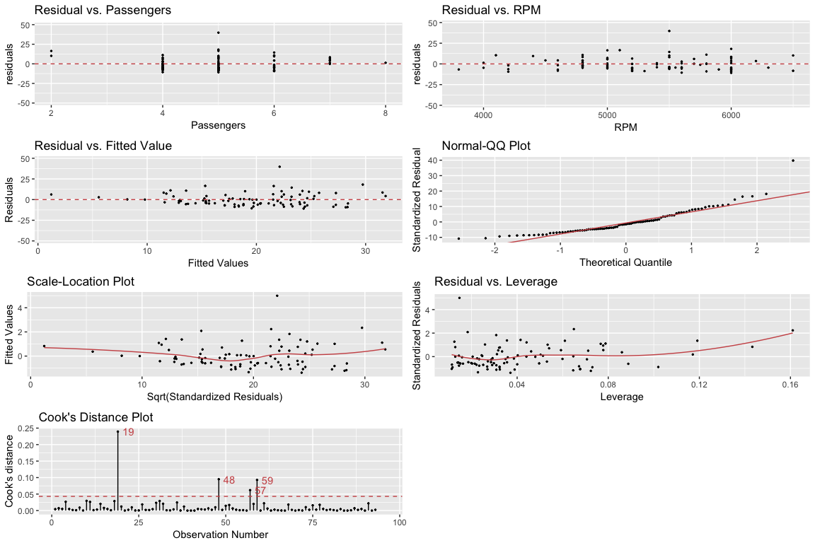
gg_resX() and gg_diagnose() would return multiple plots after a call to the function. By default, they would return one aggregate plot of all diagnostic plots as one arranged grid. If user needs more flexibility in determining graphical elements and inclusion/exclusion of certain plots, set plot.all parameter in the function call to FALSE. It will return a list of all plots, which user can manipulate.

An example would as be followed:

plots <- gg_diagnose(cars_lm, plot.all = FALSE)
names(plots)
#  [1] "residual_hist" "Passengers"    "Length"        "RPM"          
#  [5] "res_fitted"    "qqplot"        "scalelocation" "resleverage"  
#  [9] "cooksd"
exclude_plots <- plots[-c(1, 3)]    # exclude certain diagnostics plots
include_plots <- plots[c(1, 3)]      # include certain diagnostics plots

In addition, lindia provides a plot_all() feature that allows user to pass in a list of plots and output as a formatted grid of plots using gridExtra::grid.arrange().

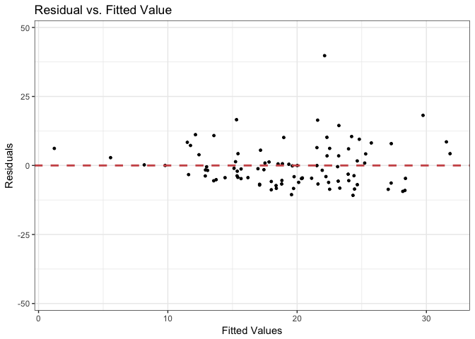
plot_all(exclude_plots)

All graphical styles returned by lindia graphing function can be overwritten by a call to ggplot::theme() (except gg_resX() and gg_diagnose(), which would return a list rather than a single ggplot object).

gg_resfitted(cars_lm) + theme_bw()

Functions in Lindia

The following gives a brief demonstration of how to use the functions provided in lindia.

gg_reshist

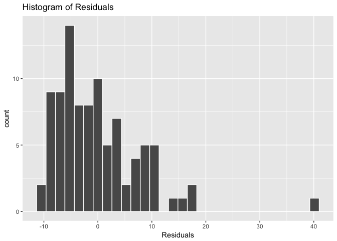
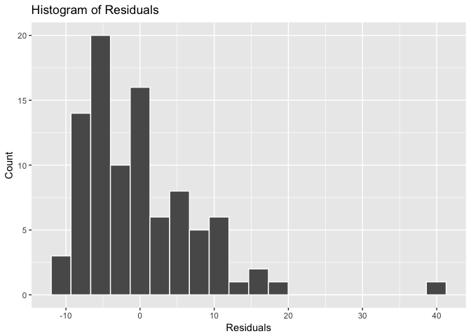
Plots distribution of residuals in histograms. Number of bins picked by default.

gg_reshist(cars_lm)

Can also specify number of bins using bins argument:

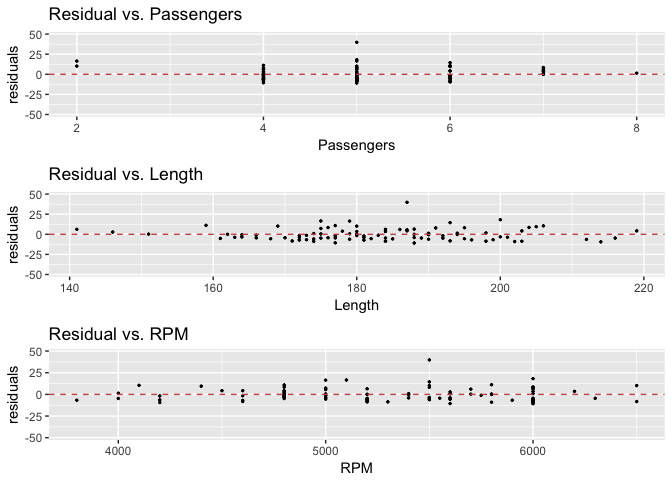
gg_reshist(cars_lm, bins = 20)

gg_resX

Plots residual plots of all predictors vs. residuals and return all plots as one plot that is arranged by package gridExtra. If a variable is continuous, it would be plotted as scatterplot. If a given variable is category is categorical, lindia would plot boxplot for that variable.

cars_lm_2 <- lm(Price ~ Passengers + Length + RPM + Origin, data = Cars93)
gg_resX(cars_lm)

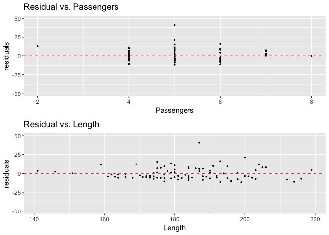
lindia can also handle linear models with interaction terms.

cars_lm_inter <- lm(Price ~ Passengers * Length, data = Cars93)
gg_resX(cars_lm_inter)

gg_resfitted

Plots residual against fitted value.

gg_resfitted(cars_lm)

gg_qqplot

Plots quantile quantile plot of a linear model, with qqline overlayed on top.

gg_qqplot(cars_lm)

gg_boxcox

Plots boxcox graph of given lm object, with labels showing optimal transforming power of response variable using box-cox transformation. Can hide labels on graph by setting showlambda to FALSE.

gg_boxcox(cars_lm)

gg_scalelocation

Plots scale location graph of linear model.

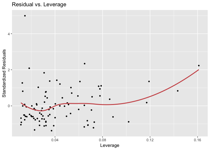
gg_scalelocation(cars_lm)

gg_resleverage

Plots residual vs. leverage of data points to detect outliers using cook's distance.

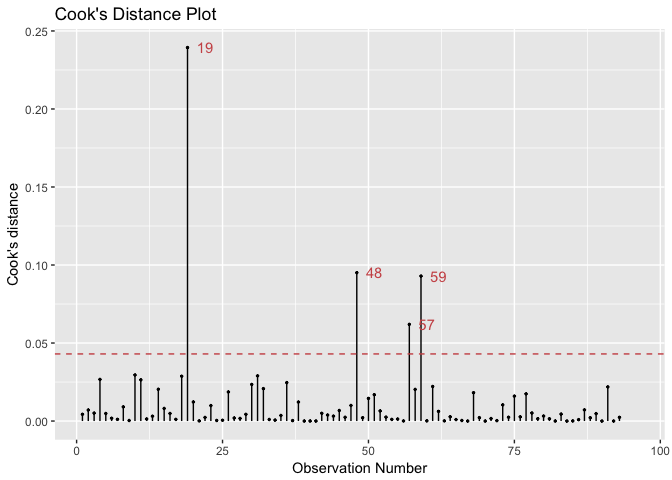
gg_resleverage(cars_lm)

gg_cooksd

Plots cook's distance plot that helps identify outliers. Observation numbers are plotted next to data points that are considered anamolies.

gg_cooksd(cars_lm)

gg_diagnose

An aggregate plot of all diagnostics plots, layed out on one panel as demonstrated in the beginning of this README document. User can set theme parameter to a specific theme type in order to apply to all plots in the panel.

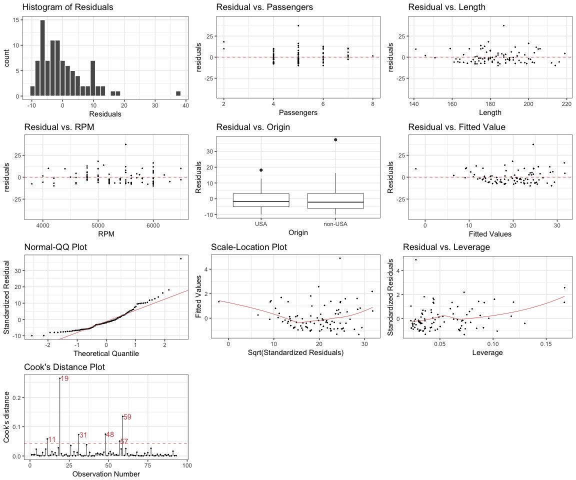
gg_diagnose(cars_lm_2, theme = theme_bw())

If user set plot.all parameter to false, gg_diagnose would return a list of ggplot objects which user can manipulate. lindia also provides a handy trick that allows user to scale all point sizes and linewidth at once, using the parameter scale.factor. Followed is an extreme example by setting scale.factor to 0.3.

gg_diagnose(cars_lm_2, theme = theme_bw(), scale.factor = 0.3)

Package Dependency

Lindia is built on top of the following few packages:

ggplot2: ver 2.1.0
gridExtra: ver 2.1.1

yeukyul/lindia