XPPAUT is a great software for the analysis of dynamical systems. Many mathematical models have been implemented with XPPAUT (*.ODE file format) [search for examples at http://senselab.med.yale.edu/modeldb/]. These implementations could be used to reproduce computational experiments and to quickly test ideas related to them. For instance, one could perform the sensitivity analysis of model’s parameters or parameters’ space searches. However, due to the graphical nature of XPPAUT, the batch modification of parameters of these models is problematic.
Here I describe the solution for this problem using simple python module Py_XPPCALL that I have written to interface with XPPAUT. It allows you to batch-modify model’s parameters and returns corresponding solutions. An analogous software exists, https://github.com/jsnowacki/xppy, however little documentation is available.
Py_XPPCALL is easy to use and does not require installation. Simply put xppcall.py to your python path or current folder.
We pay particular attention to the easy modification of input options, initial conditions, parameters, and the intuitive access to output data. In particular, within python you can:
- Modify scalar or array initial conditions
- Modify parameters and numerics options
- Grab output data for each state variable
These features allow users to take full advantage of the existing scientific libraries in python for data manipulation. In fact the abilities are virtually identical to those listed in the matlab-xpp interface website http://www2.gsu.edu/~matrhc/XPP-Matlab.html. Here they are, verbatim:
(a) If you are not an advanced XPP user, and you don't understand how to set up multi-parameter / initial condition (I.C.) range integration batch jobs in XPP, or you find doing so too fussy and prone to mistakes. You may want to vary more than 2 parameters or I.C.s. without specifying a large table of pre-determined values within XPP, or you want to allow a user to set up the ranges interactively in Matlab.
(b) Furthermore, you might want to run Matlab scripts that adaptively select parameter values or I.C.s based on the results of previous XPP integration results (e.g. parameter estimation algorithms, "shooting" methods, etc.).
(c) You can do data analysis on the integrated orbits without writing dynamic link libraries (usually in C) that are called from within your .ode script. (Some institutional installations of XPP may not have been done with the DLL option set, which can be a problem.) Also, you can take advantage of Matlab's built-in statistical tools and visualization capabilities.
(d) You don't need an X server on a Windows platform to run XPP in silent mode, so I guess these functions might make XPP a little more usable in the event that you don't have a working X server in Windows!
Please see the several python example files for syntax usage (Py_XPPCALL_Example*.py). We also comment the xppcall.py file extensively.
I extracted the ODE source code of Hodgkin-Huxley model from the example at the website of XPPAUT http://www.math.pitt.edu/~bard/bardware/tut/newstyle.html#hh. I saved it as hh.ode. I put it to the same folder where I have xppcall.py and ran python from there.
## Py_XPPCALL Example

# import some modules including Py_XPPCALL
import matplotlib.pylab as plt
import numpy as np
from xppcall import xpprun, read_pars_values_from_file

# Let's check what are the parameters of the model
pars = read_pars_values_from_file('hh.ode')
print pars
Out[]:

    {'c': '1',
     'gk': '36',
     'gl': '.3',
     'gna': '120',
     'i': '0',
     'vk': '-77',
     'vl': '-54.4',
     'vna': '50'}
# Note: XPPAUT is not case sensitive. In Py_XPPCALL, the names of parameters and variables were chosen to be in lower case.

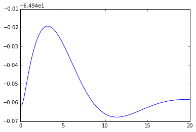
# Let's plot solution for membrane potential with parameters specified in .ODE file
npa, vn = xpprun('hh.ode', clean_after=True)
plt.figure()
plt.plot(npa[:,0], npa[:, 1+vn.index('v')])
Out[]:
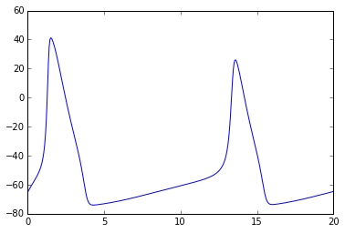
# Let's modify constant input current
npa, vn = xpprun('hh.ode', parameters={'i':20.0}, clean_after=True)
plt.figure()
plt.plot(npa[:,0], npa[:, 1+vn.index('v')])
Out[]:
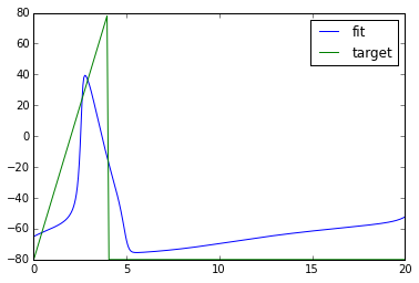
# Example of an optimization using fmin from SciPy
from scipy.optimize import fmin

# define desired V graph
target_v = -80.0+20*npa[:,0]*(np.sign(-npa[:,0]+4)+1)
plt.figure()
plt.plot(npa[:,0], target_v)
Out[]:
# define objective_func we want to minimize
def objective_func(x, target=target_v):
    try:
        npa, vn = xpprun('hh.ode', parameters={'i':x[0]}, clean_after=True)
        computed = npa[:, 1+vn.index('v')]
        return np.mean( (computed-target)**2 )
    except:
        return 1e10 # return huge error if something went wrong

xopt = fmin(objective_func, [20.0]) # find new parameters
npa, vn = xpprun('hh.ode', parameters={'i':xopt[0]}, clean_after=True)
plt.figure()
plt.plot(npa[:,0], npa[:, 1+vn.index('v')], label='fit')
plt.plot(npa[:,0], target_v, label='target')
plt.legend()
Out[]:
Congrats! We got a pretty good fit.
If you want to refer to Py_XPPCALL in a publication, you can use
"Prokin, I. and Park, Y. Py_XPPCALL. 2017. Available at: https://github.com/iprokin/Py_XPPCALL."
or BibTeX:
@misc{xppy, author = {Prokin, Ilya and Park, Youngmin}, title = {{Py_XPPCALL}}, url = {https://github.com/iprokin/Py_XPPCALL}, year = {2017} }
Ilya Prokin and Youngmin Park are equal contributors to this project.


