ML workshop for MolSim 2023

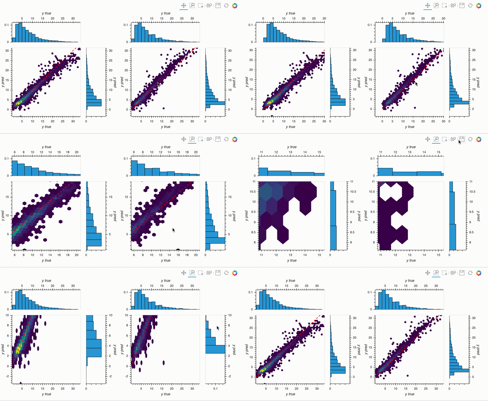
In this exercise we will build a simple model that can predict the carbon dioxide uptake in MOFs. The goal is to get familiar with the tools that are used for machine learning and to develop an understanding of the workflow, tricks, and pitfalls (e.g., why baselines are important). Some more of the theory can be found in our review.

If you find some errors, typos or issues feel free to open an issue or directly make a pull request.

How to run it

If you have a modern laptop, we recommend you run them on the laptop. If you do not want to use your machine or the cluster, you can also run the exercises on Google Colab.

Some tips

If you are not with the Python data science stack, we can recommend you some cheatsheets.
If you are not familiar with a function you can get help in a Jupyter notebook by going into the parentheses of a function and hitting SHIFT + ENTER, alternatively, you can just prepend a variable/function/library with ?, e.g., ?str.replace()
The errors you'll run into are most likely some that someone else already encountered. If you copy/paste the error message into a search engine like Google you will often find the solution to your problem on a site like StackOverflow
Here are some nice tips/tricks for using Jupyter notebooks
For plotting, we use the holoviews library as it is one of the simplest ways to create interactive figures in Python (it is a high-level interface to the bokeh library). You mind find the Getting Started section of the documentation useful if you want to understand it better. I also found this guide from Caltech useful.

Run it locally (recommended)

The following steps assume that you use MacOS or some Linux flavor. If you use Windows, we recommend that you first install the Windows Subsystem for Linux (WSL).

Create a new folder and clone this repository (you need git for this, if you get a missing command error for git you can install it with sudo apt-get install git)

git clone --depth 1 https://github.com/kjappelbaum/ml_molsim.git
cd ml_molsim

We recommend that you create a virtual conda environment on your computer in which you install the dependencies for this exercise. To do so head over to Miniconda and follow the installation instructions there.

Then, use

conda env create -f environment.yml -n ml_molsim

You can activate this environment using

conda activate ml_molsim

After this you can start Jupyter Lab and select the molsim_ml.ipynb file from the file browser.

jupyter lab

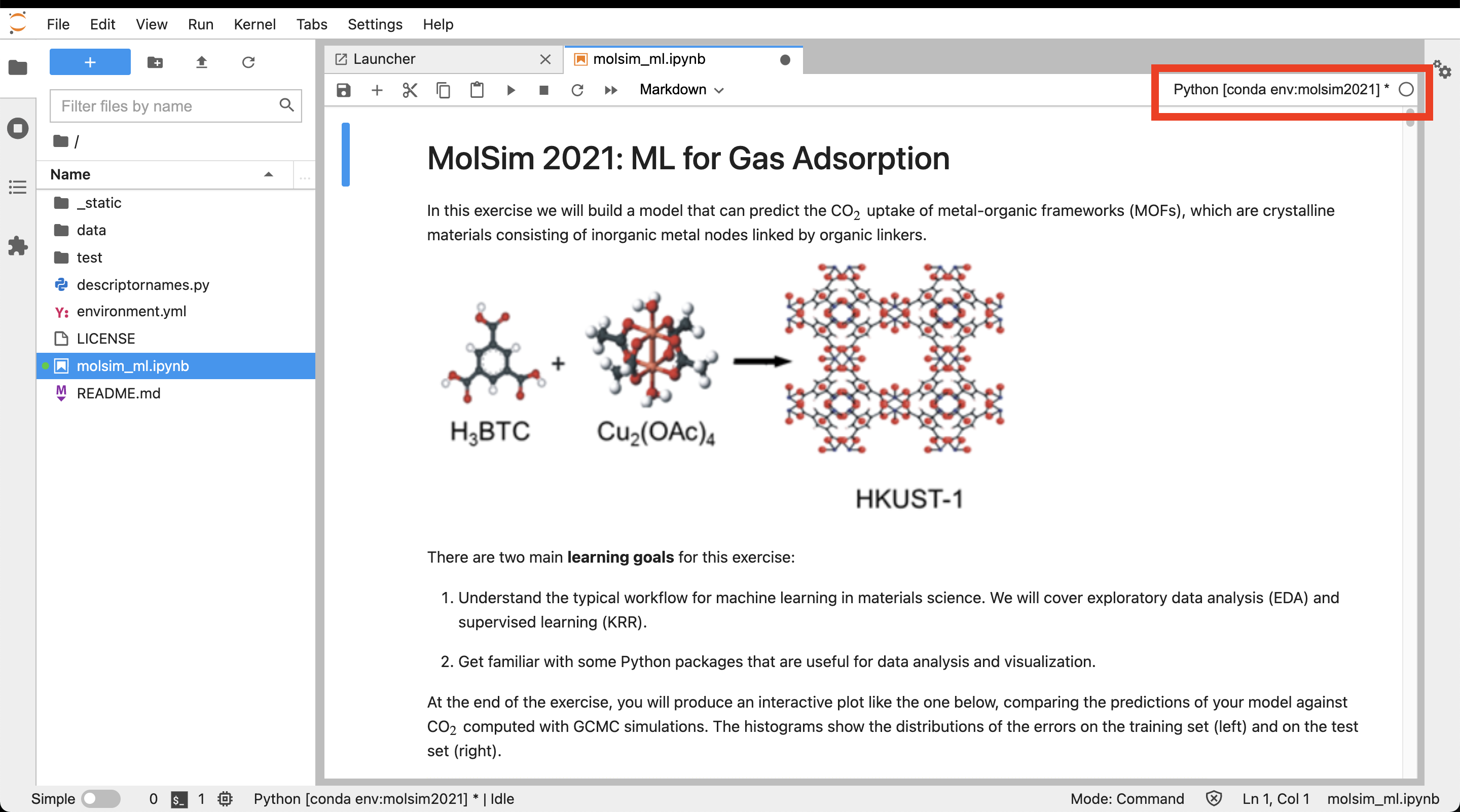
Make sure that the notebook kernel runs in the correct environment:

If the environment name that is shown is different from "ml_molsim" you can click on it and select the correct one.

Use it on Google Colab

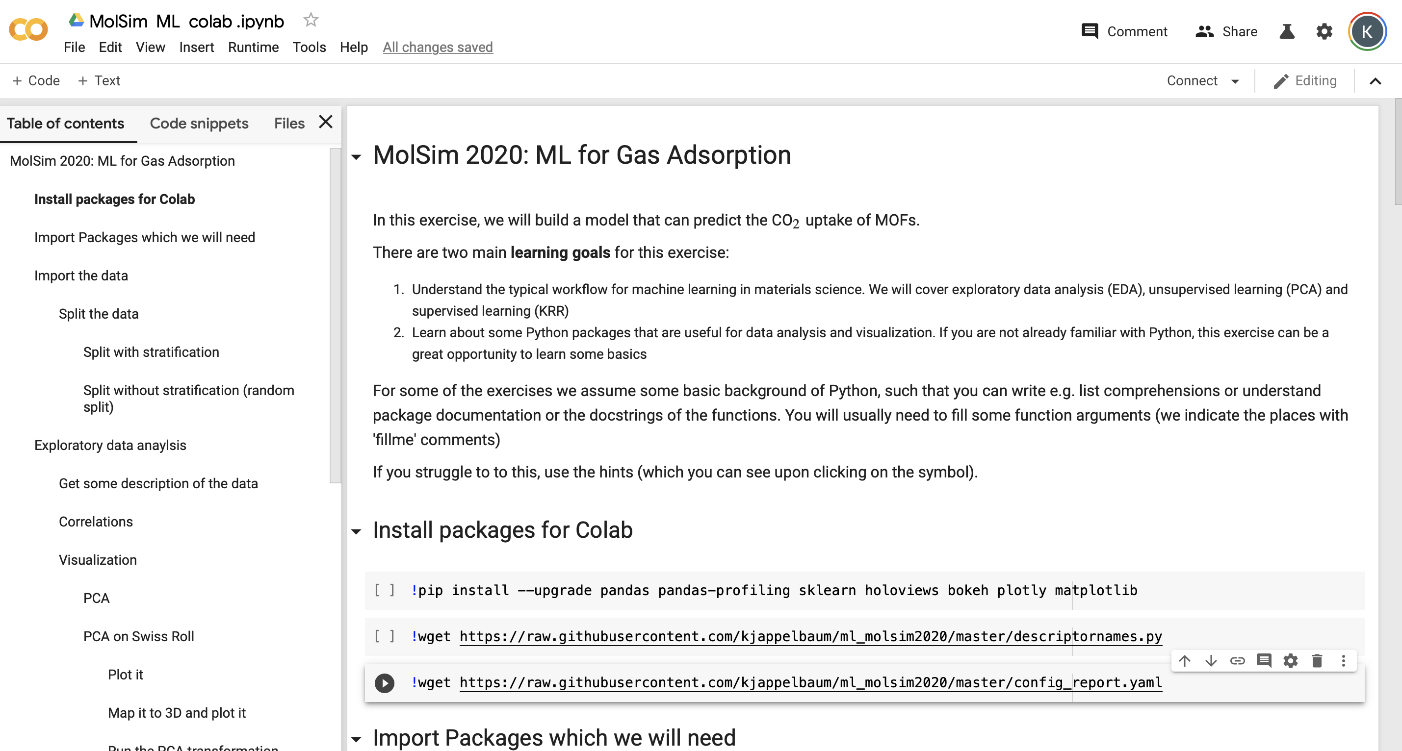
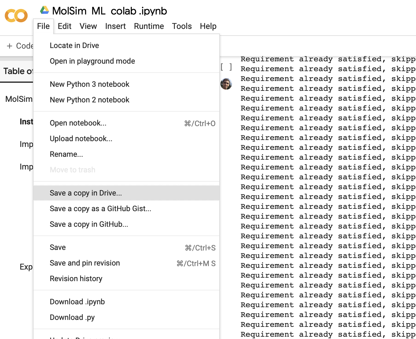
Here, you can use relatively powerful computing resources (like GPUs and TPUs) from Google for free. Click the "Open in Colab" button on the top, then make a copy of the notebook into your Google Drive, and run the first three cells to install the dependencies. Then you should be able to use the notebook in Colab.

Make sure to make a copy into your Google Drive and work on this copy. And not on the shared notebook!

Note: If you have a Google Account from your organization, e.g. university, you might need to log out and use your personal account as many organizations block third-party applications.

Note: Google Colab also requires that you reload the JavaScript of holoviews in each plotting cell. So, you have to start every cell with a holoviews plot with hv.extension('bokeh')

Acknowledgements

We want to thank Leopold Talirz for incredibly valuable feedback and input during the initial phases of development. We also want to thank Peter Alexander Knudsen for spotting typos, as well as Prof. Tristan Bereau and all MolSim participant and TAs for feedback.