Exaggerated Shading

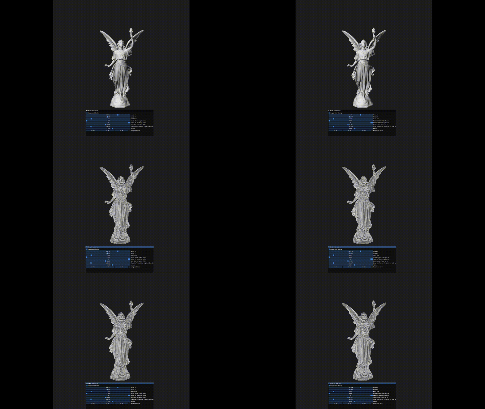
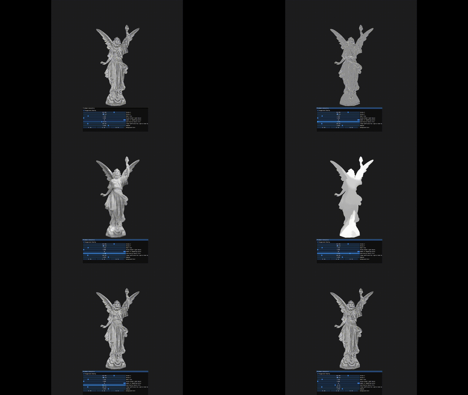
Interactive OpenGL program implementing Xshade by Szymon Rusinkiewicz, Michael Burns, and Doug DeCarlo. Exaggerated Shading for Depicting Shape and Detail. ACM Transactions on Graphics (Proc. SIGGRAPH) 25(3), July 2006.

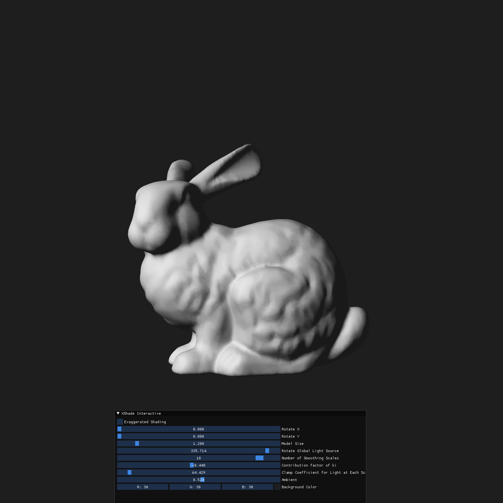
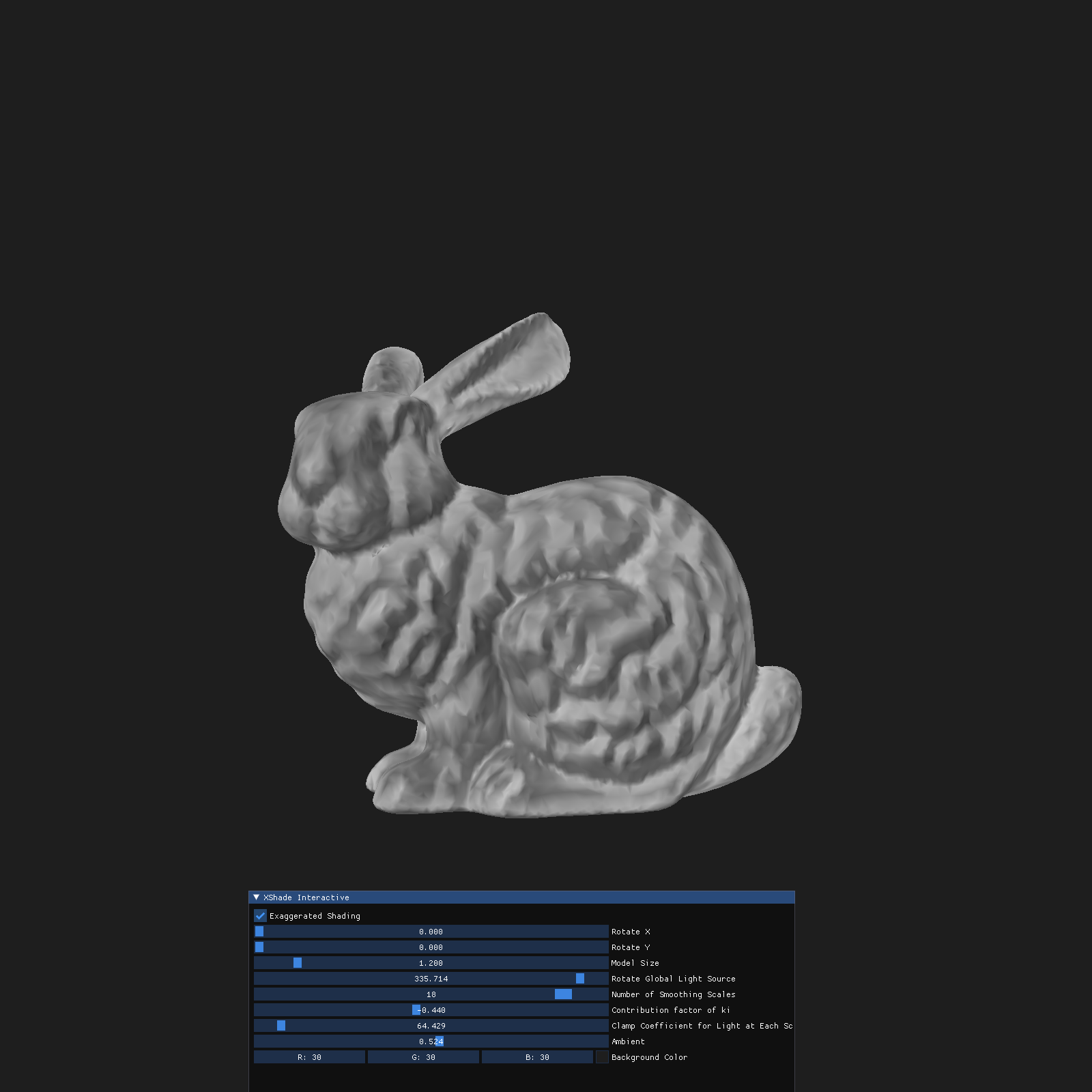
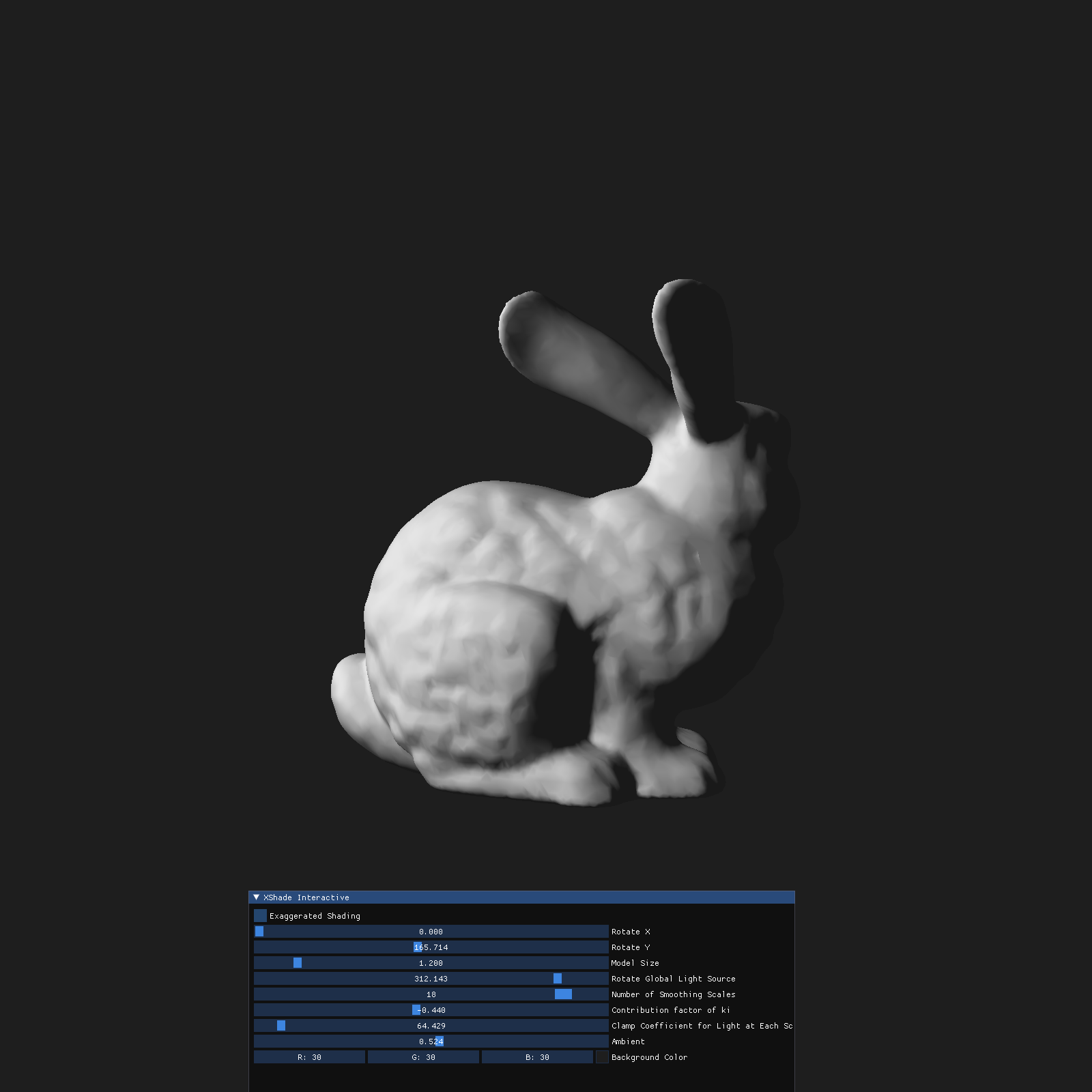
Diffuse Shading	Exaggerated Shading

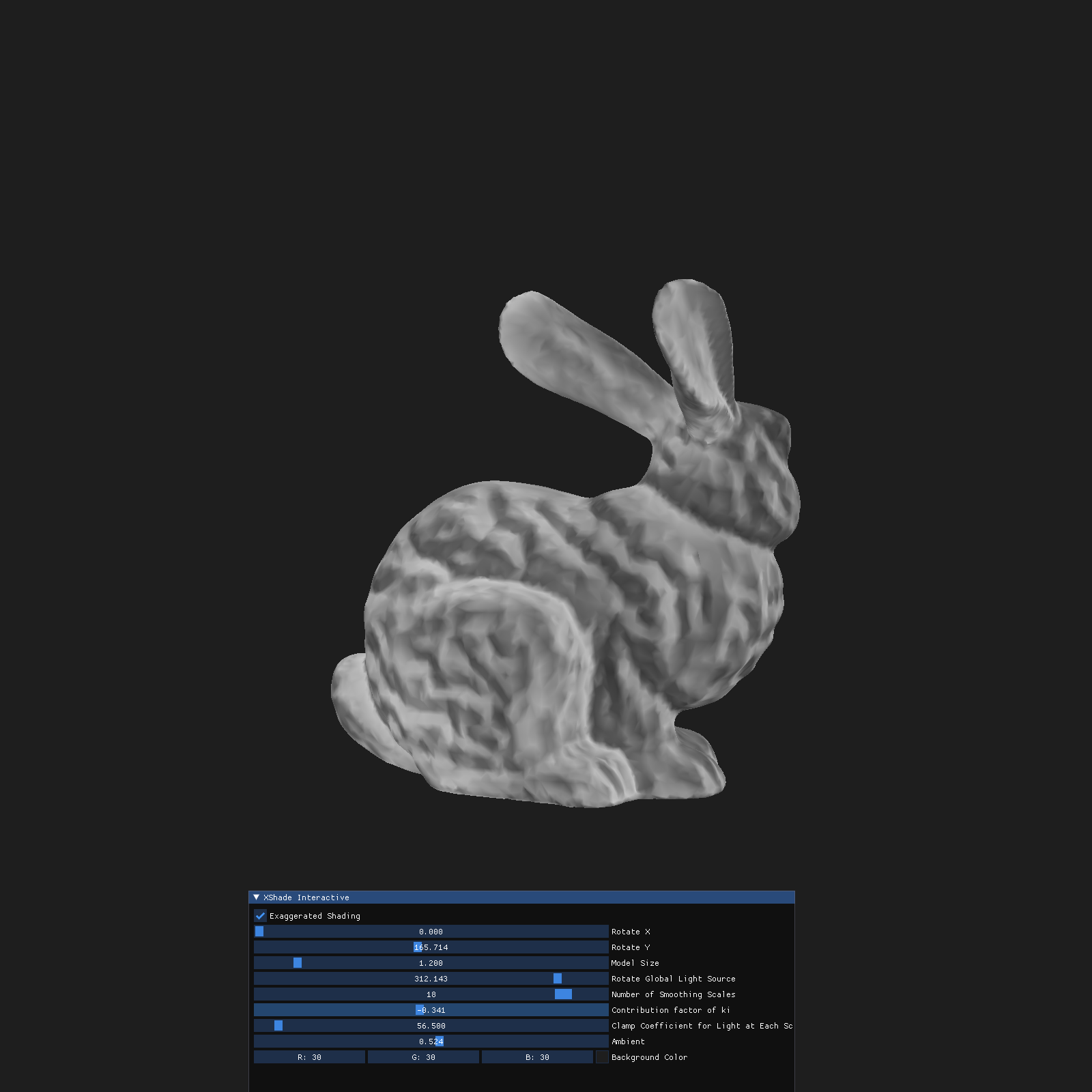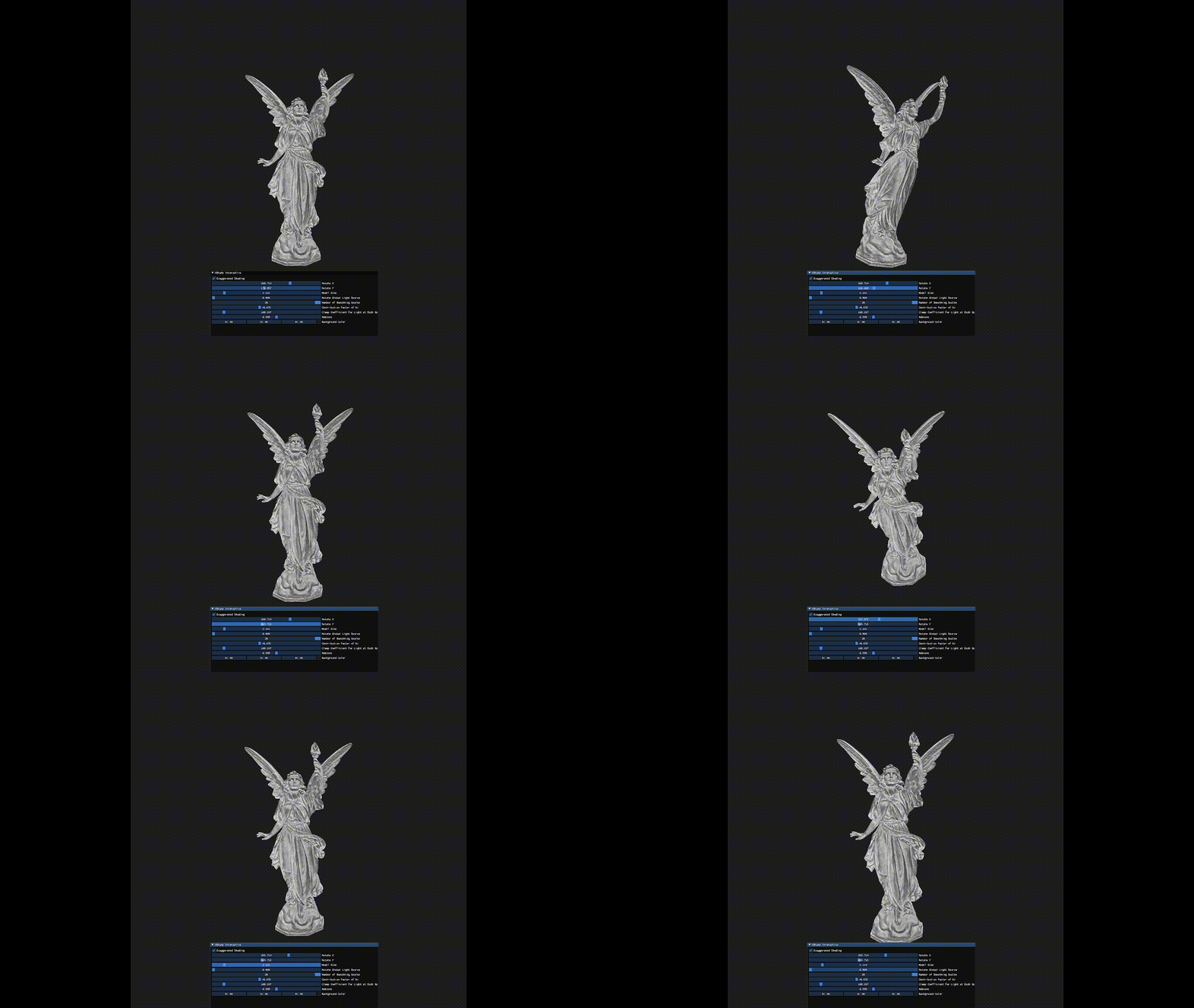
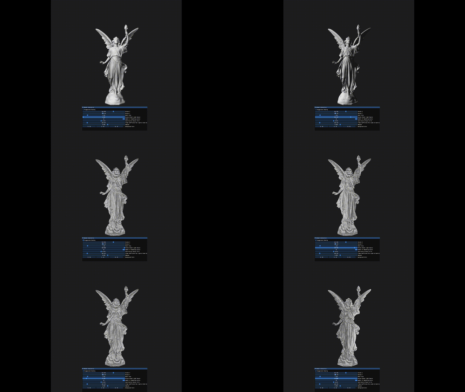
Rendering of the 3D object with exaggerated details independent of light orientation can be seen.

In a directionally lighted scene, surfaces on a 3D mesh that are alligned to or perpendicular to the light direction have a tendency of losing detail and contrast when rendered. This paper provides a shading method that reveals details at all scales.

Method

Exaggerated Shading for Depicting Shape and Detail proposes an original shading technique for revealing details at all frequencies, independent of light position and surface orientation.

This shading method is introduced as a form of "Multiscale local toon shading", and is based off of principle techniques used in cartographic terrain relief.

Key Ideas

Lighting is clamped as a cel shader to emphasize large bends, oppposeed to gradually lighted rendering. In practice we use a "smooth clamp".
Lighting is computed at multiple scales using surface normals smoothed by different amounts to convey overall shape and details at different frequencies.
Light direction varies as if it is always at a grazing position with respect to the overall orientation of that part of the object, bringing out detail of the object.

Principles of Cartographic Shaded Relief

Shadows and specular reflections are omiited.
Lighting should broadly seem to appear to originate from the top of the image. (Usually the upper left direction.)
The origin direction of light can be locally adjusted. If a mountain curves on the map, one side of the map should be uniformly light and the other uniformly dark, regardless of the orientation to the light source.
Height should be exaggerated, and ridges and valleys should have sharp transitions in brightness.
The shaded image should be a blend between the original rendering and the smoothed version.

Implementation

The shading method proposed in the paper requires several levels of smoothed normals to be preprocessed, each using a progressively larger Gaussian filter for smoothing of the normals.

For each smoothing scale, the standard deviation of the Gaussian filter is increased exponentially by a constant scalar coefficient. The paper suggests $\sqrt{2}$ for each level.

$$ \sigma_{n+1} = \sqrt{2}\sigma_n $$

As an implementation I've made a seperate repository for preprocessing and saving the smoothed normals of a 3D object at each scale using Gaussian fallout as weights.

With theses smoothed normals, the light direction is adjusted per vertex and per scale to attenuate detail at all frequencies.

The adjusted light intensity for exaggerated shading of details is implemented as below.

$c_i$ represents light at each scale.

$n_i$ is the surface normal at the current scale, and $n_{i+1}$ is the surface normal at the next smoothed frequency. $n_b$ is the normal of the "base" scale, or the scale with smallest detail.

$l_{i+1}$ is the direction of light used at each scale, and $l_{global}$ is the "global" light direction, or general light direction of the rendered scene.

$c$ is the result intensity of each vertex.

$k$ is the respective weighted "contribution" coefficient of each scale, indicating whether we want to put emphasis on scales at larger frequencies or lower frequencies. The paper suggests a contribution factor relative to an exponent of $\sigma$ at each scale. The sum of all $k$ must be unit size.

$$c_i = \underset{[-1,1]}{clamp}(a(n_i \cdot l_{i+1}))$$

$$l_{i+1} = l_{global} - n_{i+1} ( n_{i+1{}} \cdot l_{global} )$$

$$ c = \frac{1}{2} + \frac{1}{2} ( k_b (n_b \cdot l_{global}) + \sum_{i=0}^{b-1}k_i c_i ) $$

The clamp() function is used for "smooth cel shading". Used with coefficient $a$, the exaggeration factor for sending values to extreme values of -1 or 1, the clamp functions as a "smooth" version of cel shading where most values are set discretely to either -1 or 1, but still has a continuous transition through -1 and 1.

$l_{i+1}$ is calculated by projecting the global light direction onto the tangent plane of the next smoothed normal, resulting in a light with "grazing" position relative to the current normal, as in a almost perpendicular position for vertices at ridges or valleys.

Then $c$ is calculated as a weighted sum of lightings at all scales. This results in an image that displays details of the object at all detail frequencies, independent of surface orientation to the light source, similar to a map made to display terrain relief.

Principal Direction-based Light Adjustment

The basic rendering model simply projects the light source at each point into the tangent plane perpendicular to the smoothed normal. Instead with a formulization of "contrast" proposed in the paper as :

$$ contrast = || \nabla (n \cdot \delta) || $$

$n$ is the surface normal at each scale, and $\delta$ is the direction of the light source.

This is intuitively understandable as the gradient $\nabla$ indicates the direction of largest change, and the dot product $n\cdot\delta$ is what determines the diffuse factor of light intensity in shading. Thus the size of the gradient can be seen as the level of "contrast" in the rendered scene.

The paper references identities by do Carmo, 1976 that show an equivalence of this norm of gradient to :

$$ || \mathrm{II} \delta || = \sqrt{ 2H\kappa_\delta - K } $$

where $\mathrm{II}$ is the second fundamental tensor, $H$ is mean curvature, $K$ is Gaussian curvature, and $\kappa_\delta$ is the normal curvature in direction $\delta$. This is maximized when the magnitude of the normal curvature is the largest, as in when the normal curvature is in the maximum principle direction.

Therefore, we come to the conclusion that maximum contrast, by our definition, is achieved when the light sourse is positioned along the first principal direction at each point.

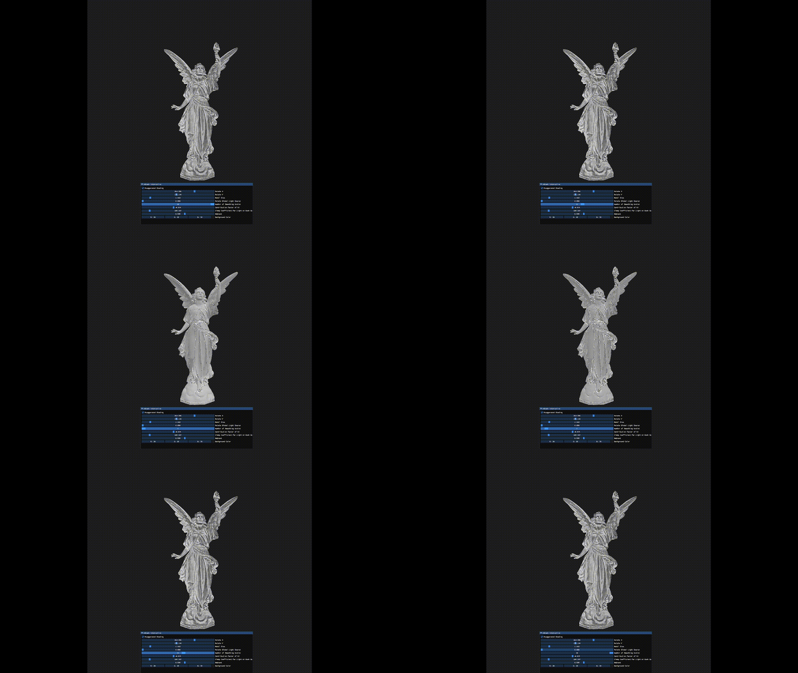
Implemented Interactive Features

The paper, published in 2006, renders these exaggerated shadings of 3D objects as images. Currently this method can be easily rendered in realtime with interactive controls for the user controlled hyperparameters provided in the paper.

Features

Switch between standard cosine shading and our exaggerated shading method.

Model rotation and size.

Rotation of "global" light direction.

Number of Smoothing Scales to use in rendering.

Exponent to $\sigma$ of the contribution factor for each scale. A low factor will make the contribution of lower frequencies larger, emphasizing small details in the image. Vice versa a higher factor will make the contribution of larger frequencies higher, emphasizing large details and making the shading more smooth and less detailed. Optimal visuals usually lie between -0.5 and -1.0.

Clamp Coefficient $a$ for the "soft cel shading" implemented with clamp(). A factor of 20~50 reveals details well in most cases.

Ambient factor added to all lighting. Default set as 0.5 in the methods proposed in the paper.

Dependencies

Written in C++ using OpenGL4 and GLFW3.

Used ImGui for interface purposes.

Used Assimp for loading 3D models.

Built using vcpkg on Windows.

yunjay/Exaggerated-Shading