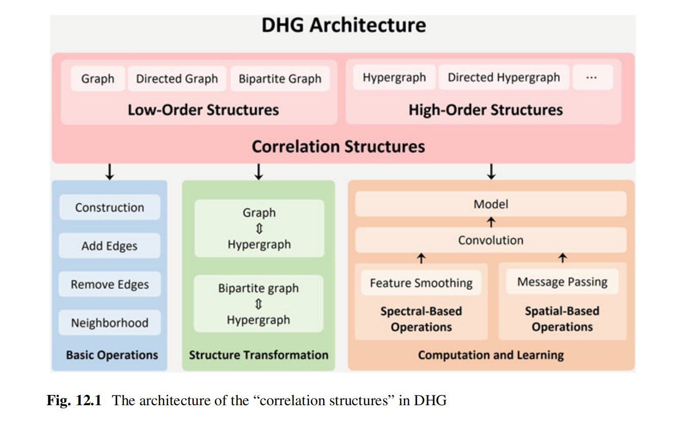
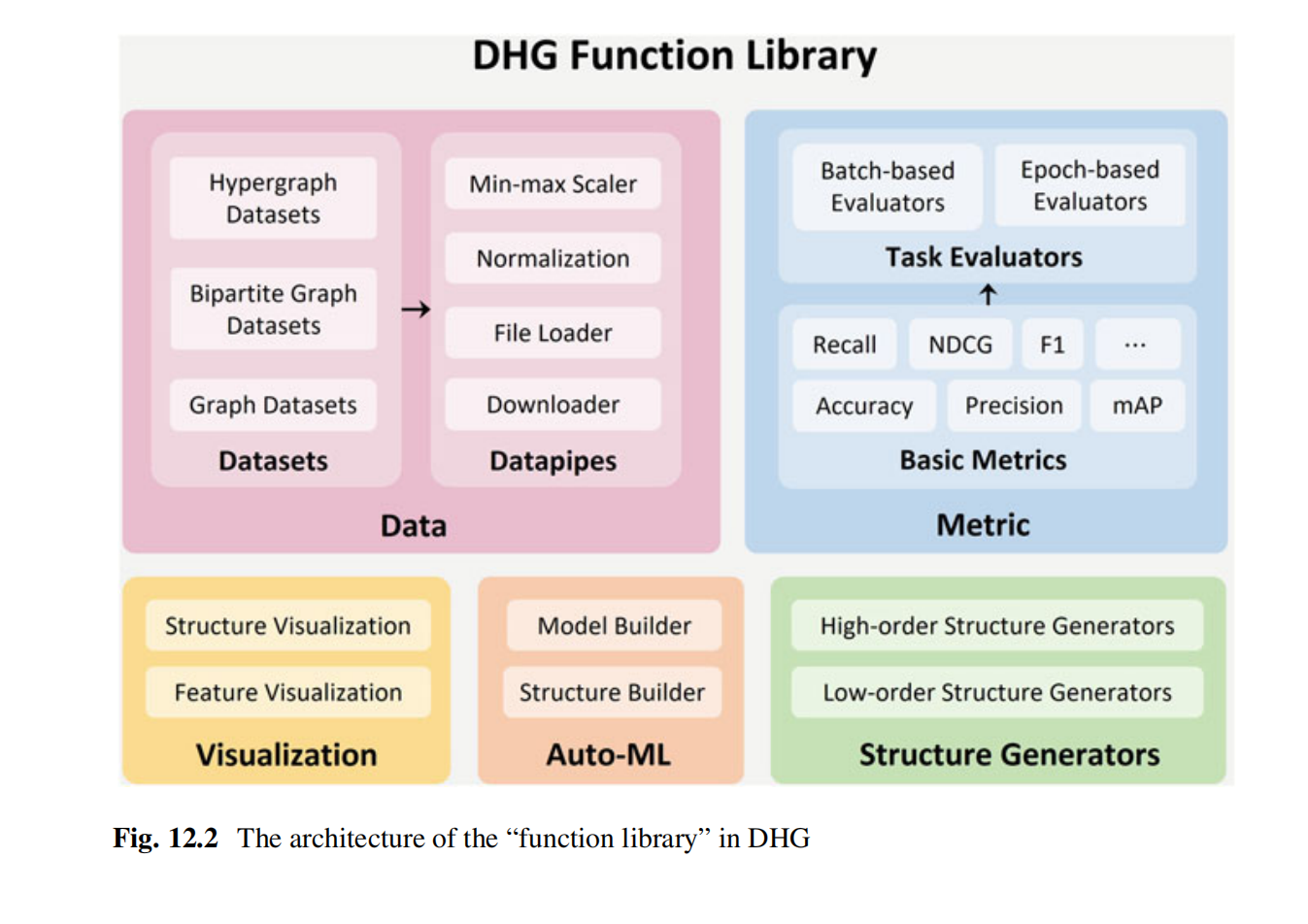
DHG(DeepHypergraph)是一个基于PyTorch的深度学习库,用于图神经网络和超图神经网络的学习。 GitHub
目前库版本的情况如下
python>=3.8
torch==1.13.1
numpy==1.24.1
安装cpu版pytorch的话,代码为
conda install pytorch==1.13.1 cpuonly -c pytorch
之后再安装dhg就可以了
pip install dhg
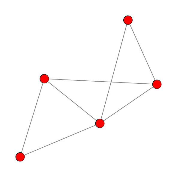
首先我们构建一个图:
# %load ./test_graph.py
import torch
import dhg
import matplotlib.pyplot as plt
# 构建图
g = dhg.Graph(5, [(0, 1), (0, 2), (1, 3), (3, 4), (0, 4), (2, 4), (1, 4)], merge_op="mean")
print(g.v)
print(g.e)
print(g.A.to_dense())

# 也可以从邻接表构建图
# g = dhg.Graph.from_adj_list(5, [[0, 1, 2], [1, 3], [4, 3, 0, 2, 1]])
# 也可以用随机方法构建图
# g = dhg.random.graph_Gnm(5, 8)
# 随机初始化一个特征矩阵
# # Generate a vertex feature matrix with size 5x2
X = torch.rand(5, 2)

# 图的可视化
g.draw()
plt.show()
[0, 1, 2, 3, 4]
([(0, 1), (0, 2), (1, 3), (3, 4), (0, 4), (2, 4), (1, 4)], [1.0, 1.0, 1.0, 1.0, 1.0, 1.0, 1.0])
tensor([[0., 1., 1., 0., 1.],
[1., 0., 0., 1., 1.],
[1., 0., 0., 0., 1.],
[0., 1., 0., 0., 1.],
[1., 1., 1., 1., 0.]])
接下来对特征进行谱方法的信息聚合
(GCN流程为
X_ = g.smoothing_with_GCN(X)
print(X_)
# # Print the inside Laplacian Matrix by GCN on the graph structure
# g.L_GCN.to_dense()
# # tensor([[0.2000, 0.2582, 0.2236, 0.2000, 0.2236],
# #         [0.2582, 0.3333, 0.0000, 0.2582, 0.0000],
# #         [0.2236, 0.0000, 0.2500, 0.2236, 0.2500],
# #         [0.2000, 0.2582, 0.2236, 0.2000, 0.2236],
# #         [0.2236, 0.0000, 0.2500, 0.2236, 0.2500]])
# # Print the vertex features after GCN-based smoothing
# X_
# # tensor([[0.5434, 0.6609],
# #         [0.5600, 0.5668],
# #         [0.3885, 0.6289],
# #         [0.5434, 0.6609],
# #         [0.3885, 0.6289]])
tensor([[0.6417, 0.6457],
[0.5446, 0.6341],
[0.4993, 0.7136],
[0.4394, 0.5295],
[0.6027, 0.8027]])
空域聚合,流程写作矩阵形式为
其中D_v:点度矩阵
# graphsage 空域聚合

X = torch.rand(5, 2)
# D_v diagnal matrix of vertex degree
# D_v^{-1}*A*X
X_ = g.v2v(X, aggr="mean")
print(X_)
tensor([[0.2214, 0.5098],
[0.5987, 0.4187],
[0.6447, 0.3750],
[0.3031, 0.5824],
[0.3784, 0.5216]])
也可以将谱域与空域聚合的信息加和
# 谱域与空域聚合的信息加和
X_ = (g.smoothing_with_GCN(X) + g.v2v(X, aggr="mean"))/2
print(X_)
tensor([[0.2906, 0.4986],
[0.5440, 0.4734],
[0.5109, 0.3512],
[0.3163, 0.5384],
[0.4156, 0.5441]])
有向图的信息传递,目前模块只提供了空域上的信息聚合,比如source to target上的信息聚合为
g = dhg.DiGraph(5, [(0, 3), (2, 4), (4, 2), (3, 1)])
X = torch.rand(5, 2)
X_src2dst = g.v2v(X, aggr="mean", direction="src2dst")
print(X_src2dst)
tensor([[0.0000, 0.0000],
[0.7418, 0.1746],
[0.4465, 0.7063],
[0.8576, 0.3098],
[0.8349, 0.0401]])
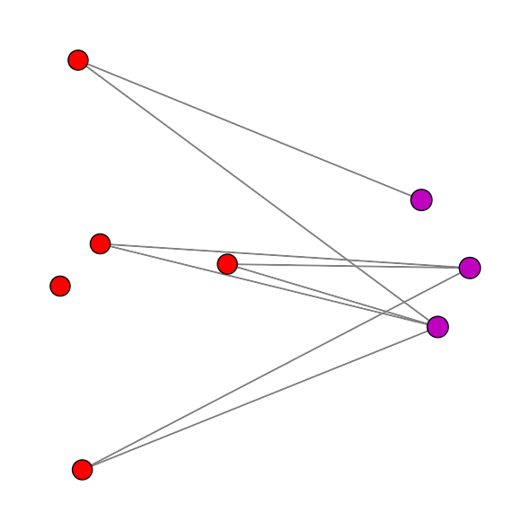
二分图(bigraph)的信息聚合
#随机初始化一个二部图,分两部U,V,节点数分别为3,5,随机生成8条边
g = dhg.random.bigraph_Gnm(3, 5, 8)


# B(3,5),B^T,稀疏U,V关联矩阵
print(g.B.to_dense())
# Generate feature matrix for vertices in set U and set V, respectively.
X_u, X_v = torch.rand(3, 2), torch.rand(5, 2)


g.draw()
plt.show()
tensor([[1., 1., 1., 0., 0.],
[1., 1., 1., 1., 0.],
[0., 0., 0., 1., 0.]])
B为U,V的bipartite adjacency matrix(3×5),相当于超图的关联矩阵
特征聚合方式为
# Propagate messages from vertices in set V to vertices in set U with mean aggregation
X_u_ = g.v2u(X_v, aggr="mean")
# Propagate messages from vertices in set U to vertices in set V with mean aggregation
# D_v^{-1} B^T X_u
X_v_ = g.u2v(X_u, aggr="mean")import torch
import dhg
hg = dhg.Hypergraph(5, [(0, 1, 2), (1, 3, 2), (1, 2), (0, 3, 4)])
print(hg.e)
print(hg.H.to_dense())
# 也可以构建随机超图,初始设定5点4边
# hg = dhg.random.hypergraph_Gnm(5, 4)
# print(hg.e)
# 随机初始化每个节点的两维特征
X = torch.rand(5, 2)([(0, 1, 2), (1, 2, 3), (1, 2), (0, 3, 4)], [1.0, 1.0, 1.0, 1.0])
tensor([[1., 0., 0., 1.],
[1., 1., 1., 0.],
[1., 1., 1., 0.],
[0., 1., 0., 1.],
[0., 0., 0., 1.]])
特别地,此模块对于由超图构建普通图,除却star与clique的方法之外,还提供了一种由超图生成图的办法,来自 HyperGCN

# 特别地,可以由hypergraph构建g
g = dhg.Graph.from_hypergraph_hypergcn(hg, X)
超图上的信息聚合也分两种,谱域上的与空域上的。
首先来看谱域上的超图图卷积流程:
其中的信息聚合
# Message propagation from hyperedge to vertex
X_ = hg.smoothing_with_HGNN(X)
空域上的信息聚合,H:
或者也可以在超边信息聚合到节点上时加上超边权重:
# X_e = D_e^{-1}H^T X_v
# 点到超边
Y_ = hg.v2e(X, aggr="mean")
# 超边到点
X_ = hg.e2v(Y_,aggr="mean")

# X_v = D_v^{-1}  H W_e X_e
# 或者也可以加上超边权重
e2v_weight = torch.rand(len(hg.e2v_weight))
X_ = hg.e2v(Y_,e2v_weight=e2v_weight,aggr="mean")

# Or, you can pass messages from vertex set to vertex set with mean aggregation by:
# 也可以直接将这个v2e,e2v两步走写成以下v2v形式
X_ = hg.v2v(X, aggr="mean")模块提供了基本图卷积层与超图卷积层的代码可供调用,具体实现就是采用模块中上述所提到的信息聚合函数,再依需要进行特征变换。
下面是一个简单的GCN卷积层的代码:
import dhg
import torch
import torch.nn as nn

class GCNConv(nn.Module):
    def __init__(
        self,
        in_channels: int,
        out_channels: int,
        bias: bool = True,
        drop_rate: float = 0.5,
    ):
        super().__init__()
        self.act = nn.ReLU(inplace=True)
        self.drop = nn.Dropout(drop_rate)
        self.theta = nn.Linear(in_channels, out_channels, bias=bias)

    def forward(self, X: torch.Tensor, g: dhg.Graph) -> torch.Tensor:
        X = self.theta(X)
        X_ = g.smoothing_with_GCN(X)
        X_ = self.drop(self.act(X_))
        return X_

g = dhg.Graph(5, [(0, 1), (0, 2), (1, 3), (3, 4), (0, 4), (2, 4), (1, 4)])
X = torch.rand(5,2)
gcn = GCNConv(2,1)
X_ = gcn(X,g)
# print(X_)
下面是一个超图节点分类的示例代码,借助了模块自带的Cooking200数据集,模型为由两个超图卷积层HGNNConv封装好的节点分类模型HGNN,损失为交叉熵损失。 模型训练与评估大同小异,我们来看其中比较核心的几句代码:
G = Hypergraph(data["num_vertices"], data["edge_list"])
net = HGNN(X.shape[1], 32, data["num_classes"], use_bn=True)
outs = net(X, G)
也就是说,我们需要输入的是超图G与初始特征矩阵X, G的确定需要节点数与超边列表(形如[(0, 1, 2), (1, 2)]),模型初始化时需要输入层的特征维数、隐藏层维数、输出层(分类层)维数,调用时输入特征矩阵X和超图G。
import time
from copy import deepcopy

import torch
import torch.optim as optim
import torch.nn.functional as F

from dhg import Hypergraph
from dhg.data import Cooking200
from dhg.models import HGNN
from dhg.random import set_seed
from dhg.metrics import HypergraphVertexClassificationEvaluator as Evaluator
def train(net, X, A, lbls, train_idx, optimizer, epoch):
    net.train()

    st = time.time()
    optimizer.zero_grad()
    outs = net(X, A)
    outs, lbls = outs[train_idx], lbls[train_idx]
    loss = F.cross_entropy(outs, lbls)
    loss.backward()
    optimizer.step()
    print(f"Epoch: {epoch}, Time: {time.time()-st:.5f}s, Loss: {loss.item():.5f}")
    return loss.item()


@torch.no_grad()
def infer(net, X, A, lbls, idx, test=False):
    net.eval()
    outs = net(X, A)
    outs, lbls = outs[idx], lbls[idx]
    if not test:
        res = evaluator.validate(lbls, outs)
    else:
        res = evaluator.test(lbls, outs)
    return res

if __name__ == "__main__":
    set_seed(2021)
    device = torch.device("cuda") if torch.cuda.is_available() else torch.device("cpu")
    evaluator = Evaluator(["accuracy", "f1_score", {"f1_score": {"average": "micro"}}])
    data = Cooking200()

    X, lbl = torch.eye(data["num_vertices"]), data["labels"]
    G = Hypergraph(data["num_vertices"], data["edge_list"])
    train_mask = data["train_mask"]
    val_mask = data["val_mask"]
    test_mask = data["test_mask"]

    net = HGNN(X.shape[1], 32, data["num_classes"], use_bn=True)
    optimizer = optim.Adam(net.parameters(), lr=0.01, weight_decay=5e-4)

    X, lbl = X.to(device), lbl.to(device)
    G = G.to(device)
    net = net.to(device)

    best_state = None
    best_epoch, best_val = 0, 0
    for epoch in range(200):
        # train
        train(net, X, G, lbl, train_mask, optimizer, epoch)
        # validation
        if epoch % 1 == 0:
            with torch.no_grad():
                val_res = infer(net, X, G, lbl, val_mask)
            if val_res > best_val:
                print(f"update best: {val_res:.5f}")
                best_epoch = epoch
                best_val = val_res
                best_state = deepcopy(net.state_dict())
    print("\ntrain finished!")
    print(f"best val: {best_val:.5f}")
    # test
    print("test...")
    net.load_state_dict(best_state)
    res = infer(net, X, G, lbl, test_mask, test=True)
    print(f"final result: epoch: {best_epoch}")
    print(res)
Epoch: 0, Time: 0.57075s, Loss: 2.99680
update best: 0.05000
Epoch: 1, Time: 0.44458s, Loss: 2.71560
Epoch: 2, Time: 0.34824s, Loss: 2.34183
Epoch: 3, Time: 0.33715s, Loss: 2.17803
Epoch: 4, Time: 0.35491s, Loss: 2.04616
Epoch: 5, Time: 0.35887s, Loss: 1.90518
Epoch: 6, Time: 0.32666s, Loss: 1.78512
Epoch: 7, Time: 0.33858s, Loss: 1.66366
Epoch: 8, Time: 0.31702s, Loss: 1.53951
Epoch: 9, Time: 0.32943s, Loss: 1.43321
Epoch: 10, Time: 0.33378s, Loss: 1.34211
Epoch: 11, Time: 0.30918s, Loss: 1.22630
Epoch: 12, Time: 0.30787s, Loss: 1.11867
Epoch: 13, Time: 0.34970s, Loss: 1.01440
Epoch: 14, Time: 0.33104s, Loss: 0.93420
Epoch: 15, Time: 0.30302s, Loss: 0.83996
Epoch: 16, Time: 0.30275s, Loss: 0.76163
Epoch: 17, Time: 0.30708s, Loss: 0.68340
update best: 0.05500
Epoch: 18, Time: 0.33452s, Loss: 0.61747
update best: 0.07000
Epoch: 19, Time: 0.31939s, Loss: 0.56980
update best: 0.08500
Epoch: 20, Time: 0.30552s, Loss: 0.50861
update best: 0.09500
Epoch: 21, Time: 0.35976s, Loss: 0.44348
update best: 0.11000
Epoch: 22, Time: 0.30756s, Loss: 0.39887
update best: 0.12000
Epoch: 23, Time: 0.31043s, Loss: 0.35758
update best: 0.13000
Epoch: 24, Time: 0.31487s, Loss: 0.32404
update best: 0.13500
Epoch: 25, Time: 0.29691s, Loss: 0.29471
Epoch: 26, Time: 0.29033s, Loss: 0.25857
update best: 0.14000
Epoch: 27, Time: 0.30515s, Loss: 0.23327
Epoch: 28, Time: 0.29754s, Loss: 0.20164
Epoch: 29, Time: 0.35460s, Loss: 0.18018
Epoch: 30, Time: 0.30009s, Loss: 0.16439
Epoch: 31, Time: 0.29091s, Loss: 0.14320
Epoch: 32, Time: 0.32527s, Loss: 0.12419
Epoch: 33, Time: 0.29964s, Loss: 0.11924
Epoch: 34, Time: 0.30927s, Loss: 0.10919
update best: 0.15000
Epoch: 35, Time: 0.29960s, Loss: 0.09785
update best: 0.15500
Epoch: 36, Time: 0.30507s, Loss: 0.09012
Epoch: 37, Time: 0.29983s, Loss: 0.08261
Epoch: 38, Time: 0.27957s, Loss: 0.07587
Epoch: 39, Time: 0.28515s, Loss: 0.07044
Epoch: 40, Time: 0.28125s, Loss: 0.06598
Epoch: 41, Time: 0.28380s, Loss: 0.06401
Epoch: 42, Time: 0.30753s, Loss: 0.05707
Epoch: 43, Time: 0.34185s, Loss: 0.05931
update best: 0.16500
Epoch: 44, Time: 0.30149s, Loss: 0.05196
Epoch: 45, Time: 0.29131s, Loss: 0.05082
Epoch: 46, Time: 0.28986s, Loss: 0.05012
Epoch: 47, Time: 0.30059s, Loss: 0.04576
Epoch: 48, Time: 0.29840s, Loss: 0.04435
Epoch: 49, Time: 0.30359s, Loss: 0.04230
Epoch: 50, Time: 0.29037s, Loss: 0.04270
Epoch: 51, Time: 0.29047s, Loss: 0.04103
Epoch: 52, Time: 0.28586s, Loss: 0.04028
Epoch: 53, Time: 0.30024s, Loss: 0.04073
Epoch: 54, Time: 0.30922s, Loss: 0.04037
update best: 0.17500
Epoch: 55, Time: 0.29788s, Loss: 0.03870
update best: 0.18000
Epoch: 56, Time: 0.30937s, Loss: 0.03931
update best: 0.18500
Epoch: 57, Time: 0.31250s, Loss: 0.03899
update best: 0.20000
Epoch: 58, Time: 0.29095s, Loss: 0.03811
update best: 0.23000
Epoch: 59, Time: 0.28320s, Loss: 0.03616
update best: 0.24000
Epoch: 60, Time: 0.34368s, Loss: 0.03745
update best: 0.24500
Epoch: 61, Time: 0.27734s, Loss: 0.03472
Epoch: 62, Time: 0.30756s, Loss: 0.03635
Epoch: 63, Time: 0.30114s, Loss: 0.03429
Epoch: 64, Time: 0.29200s, Loss: 0.03394
Epoch: 65, Time: 0.28902s, Loss: 0.03186
Epoch: 66, Time: 0.28697s, Loss: 0.03094
update best: 0.25000
Epoch: 67, Time: 0.30515s, Loss: 0.03513
update best: 0.27000
Epoch: 68, Time: 0.29123s, Loss: 0.03170
update best: 0.28000
Epoch: 69, Time: 0.32443s, Loss: 0.03075
update best: 0.29000
Epoch: 70, Time: 0.31617s, Loss: 0.03026
update best: 0.30500
Epoch: 71, Time: 0.31604s, Loss: 0.02878
update best: 0.32500
Epoch: 72, Time: 0.32258s, Loss: 0.02952
update best: 0.34000
Epoch: 73, Time: 0.29982s, Loss: 0.02851
update best: 0.35000
Epoch: 74, Time: 0.31248s, Loss: 0.02806
Epoch: 75, Time: 0.28563s, Loss: 0.02752
update best: 0.35500
Epoch: 76, Time: 0.28265s, Loss: 0.02637
update best: 0.36500
Epoch: 77, Time: 0.29957s, Loss: 0.02755
update best: 0.37500
Epoch: 78, Time: 0.29673s, Loss: 0.02571
update best: 0.40000
Epoch: 79, Time: 0.30071s, Loss: 0.02681
update best: 0.41000
Epoch: 80, Time: 0.30660s, Loss: 0.02745
Epoch: 81, Time: 0.29767s, Loss: 0.02608
Epoch: 82, Time: 0.29428s, Loss: 0.02521
Epoch: 83, Time: 0.29880s, Loss: 0.02618
update best: 0.43000
Epoch: 84, Time: 0.28256s, Loss: 0.02740
update best: 0.44000
Epoch: 85, Time: 0.30544s, Loss: 0.02513
Epoch: 86, Time: 0.30781s, Loss: 0.02774
update best: 0.47000
Epoch: 87, Time: 0.30798s, Loss: 0.02292
Epoch: 88, Time: 0.28853s, Loss: 0.02909
Epoch: 89, Time: 0.35561s, Loss: 0.02283
Epoch: 90, Time: 0.28191s, Loss: 0.02936
Epoch: 91, Time: 0.28398s, Loss: 0.02519
Epoch: 92, Time: 0.30105s, Loss: 0.02265
Epoch: 93, Time: 0.28409s, Loss: 0.02646
Epoch: 94, Time: 0.29564s, Loss: 0.02626
Epoch: 95, Time: 0.29017s, Loss: 0.02179
Epoch: 96, Time: 0.28142s, Loss: 0.02150
Epoch: 97, Time: 0.30784s, Loss: 0.02496
Epoch: 98, Time: 0.30202s, Loss: 0.02420
Epoch: 99, Time: 0.28663s, Loss: 0.01986
Epoch: 100, Time: 0.27743s, Loss: 0.01974
Epoch: 101, Time: 0.28717s, Loss: 0.02022
Epoch: 102, Time: 0.28923s, Loss: 0.02082
Epoch: 103, Time: 0.29163s, Loss: 0.01884
Epoch: 104, Time: 0.34017s, Loss: 0.01912
Epoch: 105, Time: 0.29264s, Loss: 0.01832
Epoch: 106, Time: 0.30278s, Loss: 0.01813
Epoch: 107, Time: 0.31264s, Loss: 0.01804
update best: 0.47500
Epoch: 108, Time: 0.28586s, Loss: 0.01819
Epoch: 109, Time: 0.28954s, Loss: 0.01744
Epoch: 110, Time: 0.29401s, Loss: 0.01901
Epoch: 111, Time: 0.29854s, Loss: 0.01822
Epoch: 112, Time: 0.29489s, Loss: 0.01862
update best: 0.48000
Epoch: 113, Time: 0.28435s, Loss: 0.01759
Epoch: 114, Time: 0.28226s, Loss: 0.01873
Epoch: 115, Time: 0.31054s, Loss: 0.01781
Epoch: 116, Time: 0.29975s, Loss: 0.01803
Epoch: 117, Time: 0.29708s, Loss: 0.01770
Epoch: 118, Time: 0.29399s, Loss: 0.01762
Epoch: 119, Time: 0.28302s, Loss: 0.01719
Epoch: 120, Time: 0.29010s, Loss: 0.01665
Epoch: 121, Time: 0.29369s, Loss: 0.01837
update best: 0.49000
Epoch: 122, Time: 0.30238s, Loss: 0.01742
Epoch: 123, Time: 0.26850s, Loss: 0.01693
Epoch: 124, Time: 0.28588s, Loss: 0.01705
Epoch: 125, Time: 0.27435s, Loss: 0.01699
Epoch: 126, Time: 0.27976s, Loss: 0.01620
Epoch: 127, Time: 0.28477s, Loss: 0.01581
Epoch: 128, Time: 0.30031s, Loss: 0.01736
Epoch: 129, Time: 0.30531s, Loss: 0.01790
Epoch: 130, Time: 0.30372s, Loss: 0.01612
Epoch: 131, Time: 0.28416s, Loss: 0.01528
Epoch: 132, Time: 0.30515s, Loss: 0.01521
Epoch: 133, Time: 0.28516s, Loss: 0.01639
Epoch: 134, Time: 0.27888s, Loss: 0.01460
Epoch: 135, Time: 0.30064s, Loss: 0.01543
Epoch: 136, Time: 0.29339s, Loss: 0.01517
Epoch: 137, Time: 0.31222s, Loss: 0.01529
Epoch: 138, Time: 0.28503s, Loss: 0.01606
Epoch: 139, Time: 0.29887s, Loss: 0.01573
Epoch: 140, Time: 0.29595s, Loss: 0.01712
Epoch: 141, Time: 0.30594s, Loss: 0.01473
Epoch: 142, Time: 0.31136s, Loss: 0.01515
Epoch: 143, Time: 0.29929s, Loss: 0.01407
Epoch: 144, Time: 0.30088s, Loss: 0.01418
Epoch: 145, Time: 0.29703s, Loss: 0.01469
Epoch: 146, Time: 0.29411s, Loss: 0.01575
Epoch: 147, Time: 0.28620s, Loss: 0.01472
Epoch: 148, Time: 0.31628s, Loss: 0.01444
Epoch: 149, Time: 0.29196s, Loss: 0.01322
Epoch: 150, Time: 0.29522s, Loss: 0.01475
Epoch: 151, Time: 0.27808s, Loss: 0.01499
Epoch: 152, Time: 0.31193s, Loss: 0.01422
Epoch: 153, Time: 0.29493s, Loss: 0.01451
Epoch: 154, Time: 0.27131s, Loss: 0.01478
Epoch: 155, Time: 0.28739s, Loss: 0.01407
Epoch: 156, Time: 0.29099s, Loss: 0.01336
Epoch: 157, Time: 0.28280s, Loss: 0.01755
Epoch: 158, Time: 0.28906s, Loss: 0.01581
Epoch: 159, Time: 0.31422s, Loss: 0.03539
Epoch: 160, Time: 0.27264s, Loss: 0.01924
Epoch: 161, Time: 0.28992s, Loss: 0.03208
Epoch: 162, Time: 0.28098s, Loss: 0.02666
Epoch: 163, Time: 0.28677s, Loss: 0.02465
Epoch: 164, Time: 0.28645s, Loss: 0.02508
Epoch: 165, Time: 0.28472s, Loss: 0.02562
Epoch: 166, Time: 0.28875s, Loss: 0.02666
Epoch: 167, Time: 0.29098s, Loss: 0.02334
Epoch: 168, Time: 0.28347s, Loss: 0.02077
Epoch: 169, Time: 0.28528s, Loss: 0.01911
Epoch: 170, Time: 0.29027s, Loss: 0.01931
Epoch: 171, Time: 0.27162s, Loss: 0.01567
Epoch: 172, Time: 0.29822s, Loss: 0.01693
Epoch: 173, Time: 0.28144s, Loss: 0.01526
Epoch: 174, Time: 0.29532s, Loss: 0.01365
Epoch: 175, Time: 0.28967s, Loss: 0.01303
Epoch: 176, Time: 0.28922s, Loss: 0.01320
Epoch: 177, Time: 0.28910s, Loss: 0.01286
Epoch: 178, Time: 0.28922s, Loss: 0.01234
Epoch: 179, Time: 0.30566s, Loss: 0.01126
Epoch: 180, Time: 0.28275s, Loss: 0.01140
Epoch: 181, Time: 0.28504s, Loss: 0.01130
Epoch: 182, Time: 0.29818s, Loss: 0.01123
Epoch: 183, Time: 0.29872s, Loss: 0.01059
Epoch: 184, Time: 0.29082s, Loss: 0.01147
Epoch: 185, Time: 0.28939s, Loss: 0.01145
Epoch: 186, Time: 0.28525s, Loss: 0.01092
Epoch: 187, Time: 0.30608s, Loss: 0.01143
Epoch: 188, Time: 0.29142s, Loss: 0.01105
Epoch: 189, Time: 0.29971s, Loss: 0.01137
Epoch: 190, Time: 0.29886s, Loss: 0.01133
Epoch: 191, Time: 0.29434s, Loss: 0.01218
Epoch: 192, Time: 0.31570s, Loss: 0.01259
Epoch: 193, Time: 0.30233s, Loss: 0.01310
Epoch: 194, Time: 0.28773s, Loss: 0.01173
Epoch: 195, Time: 0.29715s, Loss: 0.01234
Epoch: 196, Time: 0.29138s, Loss: 0.01283
Epoch: 197, Time: 0.29035s, Loss: 0.01316
Epoch: 198, Time: 0.28681s, Loss: 0.01276
Epoch: 199, Time: 0.28747s, Loss: 0.01311
train finished!
best val: 0.49000
test...
final result: epoch: 121
{'accuracy': 0.5314865112304688, 'f1_score': 0.38928599082549636, 'f1_score -> average@micro': 0.5314865057832358}
本模块提供了一种自动超参选择的方法,借助optuna模块进行实现
import torch
import torch.nn as nn
import torch.optim as optim

from dhg import Hypergraph
from dhg.data import Cooking200
from dhg.models import HGNNP
from dhg.random import set_seed
from dhg.experiments import HypergraphVertexClassificationTask as Task
from dhg.metrics import HypergraphVertexClassificationEvaluator as Evaluator
# TPE(Tree-structured Parzen Estimator)
def structure_builder(trial):
    global hg_base, g
    cur_hg: Hypergraph = hg_base.clone()
    return cur_hg


def model_builder(trial):
    return HGNNP(dim_features, trial.suggest_int("hidden_dim", 10, 20), num_classes, use_bn=True)


def train_builder(trial, model):
    optimizer = optim.Adam(
        model.parameters(),
        lr=trial.suggest_loguniform("lr", 1e-4, 1e-2),
        weight_decay=trial.suggest_loguniform("weight_decay", 1e-4, 1e-2),
    )
    criterion = nn.CrossEntropyLoss()
    return {
        "optimizer": optimizer,
        "criterion": criterion,
    }


if __name__ == "__main__":
    work_root = "./temp"
    set_seed(2022)
    device = torch.device("cuda") if torch.cuda.is_available() else torch.device("cpu")
    data = Cooking200()
    dim_features = data["num_vertices"]
    num_classes = data["num_classes"]
    hg_base = Hypergraph(data["num_vertices"], data["edge_list"])
    input_data = {
        "features": torch.eye(data["num_vertices"]),
        "labels": data["labels"],
        "train_mask": data["train_mask"],
        "val_mask": data["val_mask"],
        "test_mask": data["test_mask"],
    }
    evaluator = Evaluator(["accuracy", "f1_score", {"f1_score": {"average": "micro"}}])
    task = Task(
        work_root, input_data, model_builder, train_builder, evaluator, device, structure_builder=structure_builder,
    )
    task.run(200, 50, "maximize")
[I 2024-07-27 15:29:40,998] Logs will be saved to /home/yunping/DeepHypergraph/temp/2024-07-27--15-29-40/log.txt
[I 2024-07-27 15:29:40,999] Files in training will be saved in /home/yunping/DeepHypergraph/temp/2024-07-27--15-29-40
[I 2024-07-27 15:29:41,000] Random seed is 2022
[I 2024-07-27 15:29:41,002] A new study created in memory with name: no-name-4af9ff71-16f7-4141-ae0f-82d435f8d0b1
/tmp/ipykernel_135227/1073263904.py:25: FutureWarning: suggest_loguniform has been deprecated in v3.0.0. This feature will be removed in v6.0.0. See https://github.com/optuna/optuna/releases/tag/v3.0.0. Use suggest_float(..., log=True) instead.
lr=trial.suggest_loguniform("lr", 1e-4, 1e-2),
/tmp/ipykernel_135227/1073263904.py:26: FutureWarning: suggest_loguniform has been deprecated in v3.0.0. This feature will be removed in v6.0.0. See https://github.com/optuna/optuna/releases/tag/v3.0.0. Use suggest_float(..., log=True) instead.
weight_decay=trial.suggest_loguniform("weight_decay", 1e-4, 1e-2),
[I 2024-07-27 15:29:50,947] Trial 0 finished with value: 0.3499999940395355 and parameters: {'hidden_dim': 10, 'lr': 0.0009956704582324435, 'weight_decay': 0.00016856499028548418}. Best is trial 0 with value: 0.3499999940395355.
[I 2024-07-27 15:30:01,083] Trial 1 finished with value: 0.45500001311302185 and parameters: {'hidden_dim': 10, 'lr': 0.002348633160857829, 'weight_decay': 0.0009418378430920174}. Best is trial 1 with value: 0.45500001311302185.
[I 2024-07-27 15:30:14,278] Trial 2 finished with value: 0.5199999809265137 and parameters: {'hidden_dim': 19, 'lr': 0.0019719874263090698, 'weight_decay': 0.006221946114841155}. Best is trial 2 with value: 0.5199999809265137.
[I 2024-07-27 15:30:26,792] Trial 3 finished with value: 0.44999998807907104 and parameters: {'hidden_dim': 17, 'lr': 0.004599459949791714, 'weight_decay': 0.0045199760918655345}. Best is trial 2 with value: 0.5199999809265137.
[I 2024-07-27 15:30:39,578] Trial 4 finished with value: 0.44999998807907104 and parameters: {'hidden_dim': 19, 'lr': 0.008205190552892963, 'weight_decay': 0.0005446140912512398}. Best is trial 2 with value: 0.5199999809265137.
[I 2024-07-27 15:30:40,730] Trial 5 pruned.
[I 2024-07-27 15:30:42,082] Trial 6 pruned.
[I 2024-07-27 15:30:43,178] Trial 7 pruned.
[I 2024-07-27 15:30:44,296] Trial 8 pruned.
[I 2024-07-27 15:30:45,526] Trial 9 pruned.
[I 2024-07-27 15:30:46,888] Trial 10 pruned.
[I 2024-07-27 15:30:48,063] Trial 11 pruned.
[I 2024-07-27 15:30:51,016] Trial 12 pruned.
[I 2024-07-27 15:30:52,224] Trial 13 pruned.
[I 2024-07-27 15:30:55,971] Trial 14 pruned.
[I 2024-07-27 15:31:00,178] Trial 15 pruned.
[I 2024-07-27 15:31:12,478] Trial 16 finished with value: 0.4950000047683716 and parameters: {'hidden_dim': 15, 'lr': 0.003984478131058521, 'weight_decay': 0.0015799420199334793}. Best is trial 2 with value: 0.5199999809265137.
[I 2024-07-27 15:31:13,878] Trial 17 pruned.
[I 2024-07-27 15:31:21,833] Trial 18 pruned.
[I 2024-07-27 15:31:24,442] Trial 19 pruned.
[I 2024-07-27 15:31:25,619] Trial 20 pruned.
[I 2024-07-27 15:31:26,848] Trial 21 pruned.
[I 2024-07-27 15:31:29,631] Trial 22 pruned.
[I 2024-07-27 15:31:31,012] Trial 23 pruned.
[I 2024-07-27 15:31:33,575] Trial 24 pruned.
[I 2024-07-27 15:31:36,558] Trial 25 pruned.
[I 2024-07-27 15:31:39,112] Trial 26 pruned.
[I 2024-07-27 15:31:40,435] Trial 27 pruned.
[I 2024-07-27 15:31:43,389] Trial 28 pruned.
[I 2024-07-27 15:31:45,934] Trial 29 pruned.
[I 2024-07-27 15:31:47,491] Trial 30 pruned.
[I 2024-07-27 15:31:50,413] Trial 31 pruned.
[I 2024-07-27 15:31:51,951] Trial 32 pruned.
[I 2024-07-27 15:31:53,399] Trial 33 pruned.
[I 2024-07-27 15:31:57,840] Trial 34 pruned.
[I 2024-07-27 15:31:59,299] Trial 35 pruned.
[I 2024-07-27 15:32:01,299] Trial 36 pruned.
[I 2024-07-27 15:32:04,131] Trial 37 pruned.
[I 2024-07-27 15:32:05,559] Trial 38 pruned.
[I 2024-07-27 15:32:10,379] Trial 39 pruned.
[I 2024-07-27 15:32:12,016] Trial 40 pruned.
[I 2024-07-27 15:32:17,424] Trial 41 pruned.
[I 2024-07-27 15:32:21,310] Trial 42 pruned.
[I 2024-07-27 15:32:22,850] Trial 43 pruned.
[I 2024-07-27 15:32:26,107] Trial 44 pruned.
[I 2024-07-27 15:32:29,699] Trial 45 pruned.
[I 2024-07-27 15:32:31,229] Trial 46 pruned.
[I 2024-07-27 15:32:34,146] Trial 47 pruned.
[I 2024-07-27 15:32:38,109] Trial 48 pruned.
[I 2024-07-27 15:32:41,910] Trial 49 pruned.
[I 2024-07-27 15:32:41,989] Best trial:
[I 2024-07-27 15:32:41,991] Value: 0.520
[I 2024-07-27 15:32:41,991] Params:
[I 2024-07-27 15:32:41,992] hidden_dim |-> 19
[I 2024-07-27 15:32:41,993] lr |-> 0.0019719874263090698
[I 2024-07-27 15:32:41,994] weight_decay |-> 0.006221946114841155
[I 2024-07-27 15:32:42,057] Final test results:
[I 2024-07-27 15:32:42,058] accuracy |-> 0.523
[I 2024-07-27 15:32:42,059] f1_score |-> 0.407
[I 2024-07-27 15:32:42,060] f1_score -> average@micro |-> 0.523
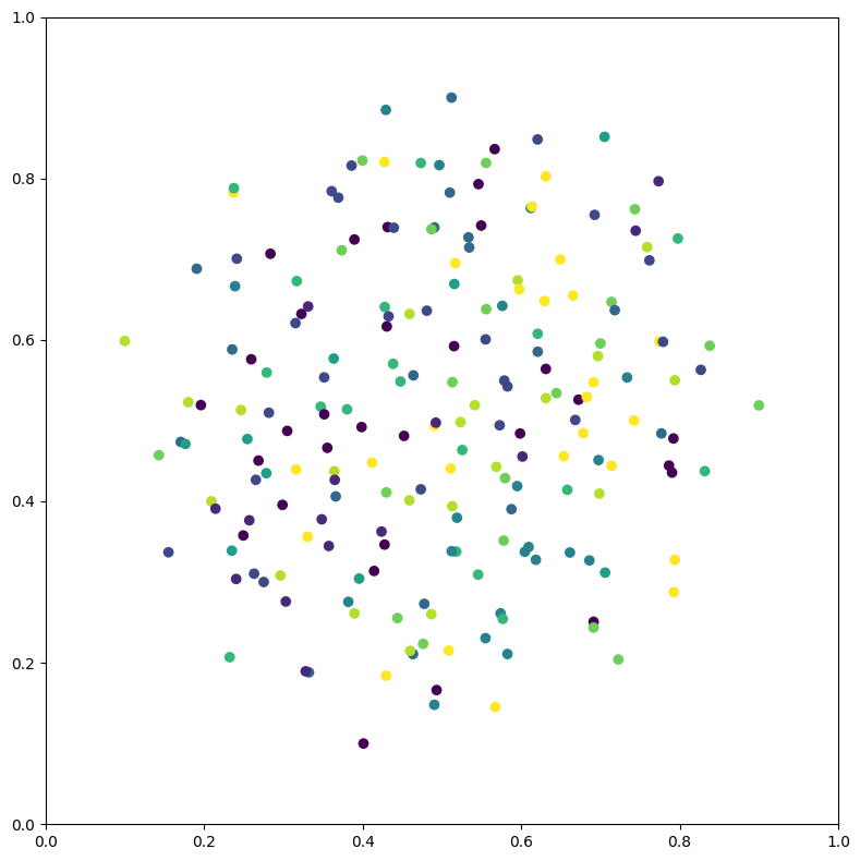
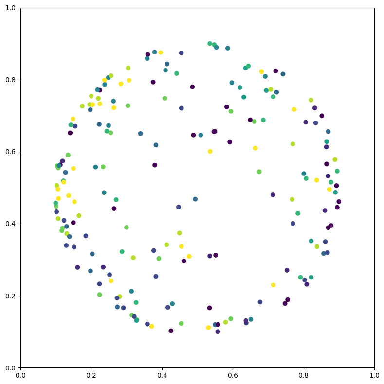
特征在欧式与双曲空间的可视化
import dhg
import numpy as np
import matplotlib.pyplot as plt
import dhg.visualization as vis
lbl = (np.random.rand(200)*10).astype(int)
ft = dhg.random.normal_features(lbl)
vis.draw_in_euclidean_space(ft, lbl)
# lbl = (np.random.rand(200)*10).astype(int)
# ft = dhg.random.normal_features(lbl)
plt.show()
vis.draw_in_poincare_ball(ft, lbl)
plt.show()